The Effects of Haze on the Accuracy of Maximum Likelihood Classification.

(1)

The Effects of Haze on the Accuracy of Maximum

Likelihood Classification

Asmala Ahmad

Department of Industrial Computing

Faculty of Information and Communication Technology Universiti Teknikal Malaysia Melaka

Melaka, Malaysia

Shaun Quegan

Department of Applied Mathematics School of Mathematics and Statistics

University of Sheffield Sheffield, United Kingdom

Copyright © 2016 Asmala Ahmad and Shaun Quegan. This article is distributed under the Creative Commons Attribution License, which permits unrestricted use, distribution, and reproduction in any medium, provided the original work is properly cited.

Abstract

This study aims to investigate the effects of haze on the accuracy of Maximum Likelihood classification. Data containing eleven land covers recorded from Landsat 5 TM satellite were used. Two ways of selecting training pixels were considered which are choosing from the haze-affected and haze-free data. The accuracy of Maximum Likelihood classification was computed based on confusion matrices where the accuracy of the individual classes and the overall accuracy were determined. The result of the study shows that classification accuracies declines with faster rate as visibility gets poorer when using training pixels from clear compared to hazy data.

Keywords: Haze, Landsat, Classification Accuracy, Training Pixels

1 Introduction

(2)

commonly used classification scheme for such purpose is Maximum Likelihood classification (ML), a supervised classification method [1], [3]. The performance of ML classification is very much influenced by the selection of the pixels used to train the ML classifier, or the so called training pixels [13]. In investigating the effects of haze on land cover classification [4], [5], there are two ways of selecting the training pixels that are to be fed to the ML classifier. The first option is selecting training pixels from the data that are affected by haze (i.e. hazy data) while the second option is selecting training pixels from the data that are free from haze (i.e. clear data). The former has been discussed in detail in [6]. We are now left to know the outcomes of the second option, i.e. selecting training pixels from clear data, in which will be addressed in this paper. Section 2 of this paper describes the methodology of the study. In section 3, the effects of haze on the classification accuracy of the individual classes are described. Section 4 discusses the effects of haze on the overall classification accuracy. Finally, section 5 concludes this study.

2 Methodology

In this study, the data comes from bands 1, 2, 3, 4, 5 and 7 of Landsat-5 TM (thematic mapper) dated 11th February 1999 and contains eleven land covers located in Selangor, Malaysia. To account for haze effects, the study made use the Landsat-5 TM datasets that have been integrated with haze layers [7], [10]. The haze layers have real haze properties with visibilities ranging from 20 km (clear) to 0 km (pure haze) [8]. Maximum Likelihood (ML) classification was performed on the hazy datasets using training pixels from the hazy and clear datasets. The reference classification to be used in this study is the ML classification of the clear dataset [6]. Accuracy assessment of the ML classification was determined by means of a confusion matrix or sometimes called an error matrix, which compares, on a class-by-class basis, the relationship between reference data (ground truth) and the corresponding results of a classification [2][3]. The three types of accuracy commonly used in measuring the performance of a classification are producer accuracy, user accuracy and overall accuracy.

Producer accuracy is a measure of the accuracy of a particular classification scheme and shows the percentage of a particular ground class that has been correctly classified. The minimum acceptable accuracy for a class is 70% [14]. This is calculated by dividing each of the diagonal elements in the confusion matrix by the total of the column in which it occurs [9]:

aa

a

c Producer accuracy

c_

 (1)

(3)

th th aa

a

c element at position a row and a column c_ column sum

 

User accuracy is another measure of how well the classification has performed. This indicates the probability that the class to which a pixel is classified from an image actually representing that class on the ground [12]. This is calculated by dividing each of the diagonal elements in the confusion matrix by the total of the row in which it occurs [9]:

aa

a

c User accuracy

c _

 (2)

where, c_a_  row sum

A measure of behaviour of the ML classification can be determined by the overall accuracy, which is the total percentage of pixels correctly classified, i.e.:

U

aa a 1

c Overall accuracy

Q





(3)

where Q and U represent the total number of pixels and classes respectively. The minimum acceptable overall accuracy is 85% [14].

The Kappa coefficient  is a second measure of classification accuracy which incorporates the off-diagonal elements as well as the diagonal terms to give a more robust assessment of accuracy than overall accuracy. This is computed as [9]:

U U

aa a a

2

a 1 a 1

U

a a

2 a 1

c c c

Q Q

c c 1

Q

 

 

  

  





(4)

where c_a row sum and ca column sum.

3 The Effects of Haze on the Producer and User Accuracy

(4)

This indicates the accuracy of the classification degrades more rapidly when using training pixels from the clear compared to hazy dataset. Compared to Figure 1(a) Some classes in Figure 1(b) reach zero accuracy at visibilities greater than 0 km visibilities. A strange trend occurs for industry at about 10 km to 6 km visibilities and 6 km to 0 km visibilities, where there is an unexpected increase in the proportion of pixels being correctly classified. We will address this issue later.

Figure 1: Producer accuracy for each class with reducing visibility when using training pixels from the hazy (a) and clear dataset (b)

Figure 2 shows the percentage of pixels for (a) coastal swamp forest, (b) dryland forest, (c) oil palm, (d) rubber, (e) cleared land, (f) sediment plumes, (g) water, (h) coconut, (i) bare land, (j) urban and (k) industry, against ground truth classes when ML classification uses training pixels from the clear dataset. 100% for a given class type, represents all the pixels from that class. There is a severe upward trend. This is due to more pixels being misclassified as visibility reduces. The main incorrect classes, which the pixels migrate to, when the visibility reduces are shown in Table 1.

Table 1: The main incorrect classes, which the pixels migrate to, as the visibility reduces. The grey shaded boxes are not relevant for this analysis

Ground Truth Pixels

Incorrect ML Class which the pixels fall in Coasta

l Swam

p Forest

Drylan d Forest

Oil Pal

m

Rubbe r

Cleare d Land

Sedimen t Plumes

Wate r

Coconu t

Bar e land

Urba n

Industr y

Coastal Swamp Forest



Drylan

(5)

Table 2: (Continued): The main incorrect classes, which the pixels migrate to, as the visibility reduces. The grey shaded boxes are not relevant for this analysis

Oil Palm   sediment plumes and industry as visibility reduces ((Figure 2(h)). A large number of coastal swamp forest pixels are misclassified as sediment plumes when the visibility drops to less than 10 km (Figure 2(a). Dryland forest pixels tend to be misclassified as cleared land and sediment plumes at shorter visibilities (Figure 2(b). At 12 km visibility, about 65% of rubber pixels are misclassified as cleared land (Figure 2(d)). About 30% of oil palm pixels are misclassified as cleared and coconut at 6 km visibility (Figure 2(c)). Urban pixels are misclassified as cleared land for visibilities less than 6 km. About 95% to 100% of non-industry pixels are misclassified as industry for visibilities 2 km and 0 km.

(6)

CSFDLF OP R CL SP W C BL U I

Figure 2: Percentage of pixels for (a) coastal swamp forest, (b) dryland forest, (c) oil palm, (d) rubber, (e) cleared land, (f) sediment plumes, (g) water, (h) coconut,

(i) bare land, (j) urban and (k) industry, against ground truth classes

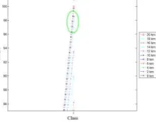
Figure 3 shows an enlarged version of Figure 2(k) associated with industry. The unusual trend is located within the green circle. The increase in the producer accuracy of industry from 6 km to 2 km is due to more pixels being correctly classified as industry at 0 km than 2 km, 4 km and 6 km visibility (

Figure 3(b)). For 0 km visibility, every pixel experiences very severe signal attenuation and scattering due to haze, eventually possesses spectral properties of the pure haze itself. Since the means and covariance structure of the pure haze pixels across the image match those of industry, consequently, most pixels are classified as industry. This risen the probability of the industry pixel being correctly classified and therefore causing ‘strange’ increase the producer accuracy. Nevertheless, spatially this is not accurate since non-industry pixels are also classified as industry; we will show this by using user accuracy measure later.

Figure 3: An enlarged version of Figure 2(k) associated with industry

(7)

(Figure 1) is not consistent with the corresponding user accuracy which is nearly zero at 0 km visibility. This indicate that most pixels on the image that are classified as industry actually does not really represent the class on the ground (spatially), e.g. urban, oil palm and forests pixels being incorrectly classified as industry.

(a) (b)

Figure 4: The user accuracies of the classes when using training pixels from the hazy (a) and clear dataset (b)

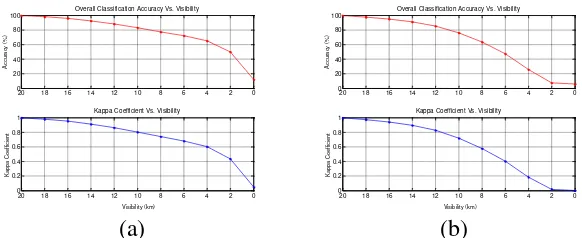
4 The Effects of Haze on the Overall Accuracy and Kappa

Coefficient

(8)

20 18 16 14 12 10 8 6 4 2 0

Overall Classification Accuracy Vs. Visibility

20 18 16 14 12 10 8 6 4 2 0

Kappa Coefficient Vs. Visibility

Visibility (km)

Overall Classification Accuracy Vs. Visibility

20 18 16 14 12 10 8 6 4 2 0

Kappa Coefficient Vs. Visibility

Visibility (km)

(a) (b)

Figure 5: Overall classification accuracy (top) and Kappa coefficient (bottom) versus visibility when training pixels are drawn from the hazy (a) and clear dataset

(b)

5 Conclusion

In this paper, we have investigated the effects of haze on the performance of the ML classification on hazy multispectral datasets. The analysis made use training pixels from hazy and clear datasets. The result shows that the decline in producer, user and overall accuracy were faster when using training pixels from clear compared to hazy datasets. This indicates the more rapid migration of pixels to incorrect classes, as visibility reduces, when using training pixels from the clear dataset. This suggests the suitability of using training pixels from a hazy dataset rather than clear dataset for performing ML classification when hazy conditions are unavoidable.

Acknowledgements. We would like to thank Universiti Teknikal Malaysia

Melaka for funding this study under FRGS Grant (FRGS/2/2014/ICT02/FTMK/02 /F00245) and Agensi Remote Sensing Malaysia for providing the data.

References

[1] A. Ahmad, Classification Simulation of RazakSAT Satellite, Procedia Engineering, 53 (2013), 472 – 482.

http://dx.doi.org/10.1016/j.proeng.2013.02.061

[2] A. Ahmad and S. Quegan, Analysis of maximum likelihood classification technique on Landsat 5 TM satellite data of tropical land covers,

Proceedings of 2012 IEEE International Conference on Control System, Computing and Engineering (ICCSCE2012), (2012), 280 – 285.

(9)

[3] A. Ahmad and S. Quegan, Comparative analysis of supervised and unsupervised classification on multispectral data, Applied Mathematical Sciences, 7 (2013), no. 74, 3681 – 3694.

http://dx.doi.org/10.12988/ams.2013.34214

[4] A. Ahmad and S. Quegan, Haze reduction in remotely sensed data, Applied Mathematical Sciences, 8 (2014), no. 36, 1755 – 1762.

[5] A. Ahmad and S. Quegan, The Effects of haze on the spectral and statistical properties of land cover classification, Applied Mathematical Sciences, 8

(2014), no. 180, 9001 – 9013.

[6] A. Ahmad and S. Quegan, The effects of haze on the accuracy of satellite land cover classification, Applied Mathematical Sciences, 9 (2015), no. 49, 2433 – 2443. http://dx.doi.org/10.12988/ams.2015.52157

[7] A. Asmala, M. Hashim, M. N. Hashim, M. N. Ayof and A. S. Budi, The use of remote sensing and GIS to estimate Air Quality Index (AQI) Over Peninsular Malaysia, GIS development, (2006), 5pp.

[8] A. Ahmad and S. Quegan, Haze modelling and simulation in remote sensing satellite data, Applied Mathematical Sciences, 8 (2014), no. 159, 7909 – 7921. http://dx.doi.org/10.12988/ams.2014.49761

[9] J. R. Jensen, Introductory Digital Image Processing: A Remote Sensing Perspective, Pearson Prentice Hall, New Jersey, USA, 1996.

[10] M. F. Razali, A. Ahmad, O. Mohd and H. Sakidin, Quantifying haze from satellite using haze optimized transformation (HOT), Applied Mathematical Sciences, 9 (2015), no. 29, 1407 – 1416.

[11] M. Hashim, K. D. Kanniah, A. Ahmad, A. W. Rasib, Remote sensing of tropospheric pollutants originating from 1997 forest fire in Southeast Asia,

Asian Journal of Geoinformatics, 4 (2004), 57 – 68.

[12] M. Story and R. Congalton, Accuracy assessment: a user's perspective,

Photogrammetric Engineering and Remote Sensing, 52 (1986), 397 – 399.

(10)

[14] J. R. Thomlinson, P. V. Bolstad, and W. B. Cohen, Coordinating methodologies for scaling landcover classifications from site-specific to global: steps toward validating global map products, Remote Sensing of Environment, 70 (1999), 16 – 28.

http://dx.doi.org/10.1016/s0034-4257(99)00055-3