Analysis of Landsat 5 TM Data of Malaysian Land Covers Using ISODATA Clustering Technique.

Analysis of Landsat 5 TM Data of Malaysian Land

Covers Using ISODATA Clustering Technique

Asmala Ahmad

Department of Industrial Computing

Faculty of Information and Communication Technology Universiti Teknikal Malaysia Melaka (UTeM)

Hang Tuah Jaya, Melaka, Malaysia asmala@utem.edu.my

Suliadi Firdaus Sufahani

Department of Science and Mathematics

Faculty of Science, Technology and Human Development Universiti Tun Hussein Onn Malaysia (UTHM)

Batu Pahat, Johor, Malaysia app08sfs@ shef.ac.uk

Abstract— This study presents a detailed analysis of Iterative Self

Organizing Data Analysis (ISODATA) clustering for

multispectral data classification. ISODATA is an unsupervised classification method which assumes that each class obeys a multivariate normal distribution, hence requires the class means and covariance matrices for each class. In this study, we use ISODATA to classify a diverse tropical land covers recorded from Landsat 5 TM satellite. The classification is carefully examined using visual analysis, classification accuracy, band correlation and decision boundary. The results show that ISODATA is able to detect eight classes from the study area with 93% agreement with the reference map. The behavior of mean and standard deviation of the classes in the decision space is believed to be one of the main factors that enable ISODATA to classify the land covers with relatively good accuracy.

Keywords- ISODATA, Landsat, Classification

I. INTRODUCTION

Studies on classification of remote sensing data have long been carried out by numerous researchers worldwide, with more efforts made regionally than globally. Many regional studies have been carried out in places such as Europe and America [1] due to having an up-to-date remote sensing facilities as well as ground truth information. There is also an increasing interest to carry out such studies in climate-affected regions such as Africa [2] and highly populated regions such as India and China [3]. Nonetheless, not much effort has been expended in Tropical countries such as Malaysia [4], [5] despite their recent promising developments in remote sensing capabilities [6]. Two types of methods that are commonly used are supervised and unsupervised classification. Supervised classification classifies pixels based on known properties of each cover type; therefore it requires representative of land cover information, in terms of training pixels. On the other hand, in unsupervised classification, the clustering process produces clusters that are statistically separable, giving a natural grouping of the pixels. This approach is useful when reliable training data are either limited or expensive, and when there is insufficient a priori information about the data [7]. Two types of commonly used unsupervised classification are

K-means and ISODATA. K-means is a simple clustering procedure that attempts to find the cluster centres in the data, then aims to cluster the full set of pixels into K clusters. The main disadvantage is that K-means requires the number of clusters is known a priori [8]. The main advantage of ISODATA over K-means algorithm is that ISODATA allows different numbers of clusters (ranging from a minimum to a maximum number of clusters) to be specified [8]; therefore is more adaptable and flexible than K-means.This study presents a detailed analysis of ISODATA clustering for Malaysian land covers using Thematic Mapper (TM), a medium resolution multispectral sensor on board Landsat 5 satellite. This makes use qualitative and quantitative approaches. Hopefully, this analysis, although limited to a single scene, will provide some insight in application of ISODATA on multispectral image classification.

II. LANDSAT SATELLITE

One of the most common remote sensing satellites is Landsat, initiated by NASA (National Aeronautical and Space Administration) in 1972 [9]. The Landsat satellites have been providing optical data for almost 40 years. In this study, we make use the Landsat 5 TM data; the satellite was launched on March 1, 1984 and is the longest running satellite of the series. The Landsat 5 satellite specifications are given in Table 1.

Table 1. Landsat 5 TM satellite specifica tions [9].

Parameter Description Spectral Bands 4 VNIR, 2 SWIR, 1 thermal Spatial Resolution (IFOV) 30 m – VNIR, SWIR

120 m – thermal Sampling 1 samples/IFOV along scan Cross Track Coverage 185 km Radiometric Resolution 8 bits

Radiometric Calibration Internal lamps, shutter and black body Scanning Mechanism Bidirectional Scanning with Scan Line

Corrector Period of Operation Landsat 5: 1984 – present

Main Sensor TM

Altitude 705 km

Repeat Cycle 16 days Equatorial Crossing 9:45 AM +/- 15 minutes

Type Sun synchronous, near polar

Inclination 98.2°

Landsat 5 TM level 1 data come in Product Generation System (LPGS) format and need to be converted into a physically meaningful common radiometric unit, representing the at-sensor spectral radiance. The Level 1 Landsat 5 TM

where, L is the spectral radiance at the sensor's aperture (W/ m2 sr m), Qcal is the quantized calibrated pixel value,

m) and L_max is the spectral at-sensor radiance that is scaled

to Q_{cal max} (W/ m2 sr m). Q_{cal min} and Q_{cal max} are 1 and 255 respectively.

Scene-to-scene variability can be reduced by converting the at-sensor spectral radiance to top-of-atmosphere (TOA) reflectance, also known as in-band planetary albedo. By performing this conversion, the cosine effect of different solar zenith angles due to the time difference between data acquisitions is removed. Different values of the exoatmospheric solar irradiance arising from spectral band differences are compensated and the variation in the Earth– Sun distance between different data acquisition dates is corrected. The TOA reflectance can be computed by using http://ssd.jpl.nasa.gov/?horizons or can be obtained from the literature (e.g. [10]). Conversion to at-sensor spectral radiance and TOA reflectance can be performed by using built-in tools in high-end image processing software.

III. ISODATACLUSTERING

The ISODATA algorithm is one of the most frequently used methods in unsupervised classification and normally assumes that each class obeys a multivariate normal distribution, hence requires the class means and covariance matrices for each class. It follows an iterative procedure and is often referred to as an extension of the K-means algorithm. The K-means is a simple clustering procedure that attempts to find the cluster centres in the data, then aims to cluster the full set of pixels into K clusters. Initially, both approaches assign arbitrary cluster centres and the cluster means and covariances are calculated. Each pixel is then classified to the nearest cluster. New cluster means and covariances are then calculated based on all the pixels in that cluster. This process is repeated until the change between iterations is “small enough”. The change can be quantified either by measuring the distances the cluster mean has changed from one iteration to the next or by the percentage of pixels that has changed between iterations. The main difference between ISODATA and the K-means algorithm is ISODATA allows different numbers of clusters (ranging from a minimum to a maximum number of clusters) to be specified, while K-means assumes the number of clusters is known a priori [8]. In more detail, the steps in ISODATA clustering are as follows:

1. Enter number of clusters.

2. The clustering first selects arbitrary initial cluster centres and then distributes the pixels among the cluster centres (i.e. a new class mean is calculated):

( )

the new cluster mean and covariance are calculated.

IV. CLASSIFICATION USING ISODATA

The study area was located in Selangor, Malaysia, covering approximately 840 km2 within longitude 101° 10’ E to 101°30’ E and latitude 2°99’ N to 3°15’ N. The satellite data come from bands 1, 2, 3, 4, 5 and 7 of Landsat-5 TM dated 11th February 1999 (Figure 1(b)). The data was chosen because have minimal cloud and free from haze, which normally occurs at the end of the year [11]. Prior to any data processing, the cloud and its shadow were masked out based on threshold approach [12]. Visual interpretation of the Landsat data was then performed, aided by a reference map (Figure 1(a)), produced in October 1991 using ground surveying and SPOT satellite data by the Malaysian Surveying Department and Malaysian Remote Sensing Agency. 11 main classes identified were water, coastal swamp forest, dryland forest, oil palm, rubber, industry, cleared land, urban, sediment plumes, coconut and bare land. Before carrying out ISODATA clustering, the number of clusters we needs to be defined here use values from 5 to 12. After the clustering process ended, the clusters were manually labelled to the nearest match, based on the reference image (Figure 1(b)). ISODATA clustering generates a cluster map with clusters assigned to arbitrary colours. In the labelling process, each cluster is matched to a class (or classes) from the reference image and given a specific colour so that at the end of the labelling process, classes (i.e. single or multiple) that exist in the cluster map can be easily recognised by their colours. This is performed for all the cluster maps. An attempt was made to match as many classes as possible to the clusters produced by the ISODATA clustering, but only 8 were found to sensibly match the clusters. They are water, coastal swamp forest, dryland forest, sediment plumes, industry, cleared land, oil palm and urban.

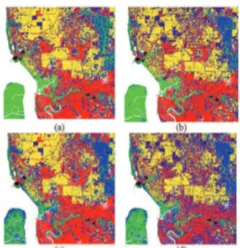
Figure 1. The study area from (a) the land cover map and (b) the Landsat-5 TM bands 5, 4, 3 assigned to the red, green blue channels.

After the merging process, the 9-, 10-, 11-, and 12- cluster maps (Figure 2 (a) to (d)) contain 8 clusters which were assigned to the urban (red), bare land (grey), oil palm (yellow), dryland forest (blue), coastal swamp forest (green), cleared land (dark purple), sediment plumes (sea green) and water (white) classes.

Figure 2. (a) 9-, (b) 10-, (c) 11- and (d) 12- cluster maps that possess 8 clusters after cluster merging.

It is noticeable that in the 9-cluster map some portions of dryland forest are being classified as coastal swamp forest, while in the 11- and 12- cluster maps some portions of coastal swamp forest are classified as dryland forest. The 10-cluster map (Figure 2(b)) is able to cluster the pixels that correspond to the major classes (viz. water, coastal swamp forest, dryland forest, oil palm, cleared land, bare land, urban and sediment plumes) better than other cluster maps, thus is more preferable. Nevertheless, three classes cannot be detected by the ISODATA clustering. They are rubber, coconut and bare land; this is due to the fact that these classes are statistically similar with other classes that they tend to merge with those classes.

Figure 3 is the enlarged version of Figure 2(b); coastal swamp forest and dryland forest can be clearly seen in the south-west and north-east of the classified image, as indicated by the reference map. Coastal swamp forest covers most of the Island and coastal regions in the south-west of the scene. Most of the dryland forest can be recognised as a large straight-edged region in the north-east. Oil palm dominates the northern parts while urban the southern parts. Industry can be recognised as patches near the urban areas, especially in the south-west and north-east. A quite large area of cleared land can be seen in the northern parts and seems to be surrounded by the oil palm. Sediment plumes can be seen on the northwest of the image. The area of the detected classes in km and percentage is given in Table 2. The biggest class is oil palm (300 km2), followed by cleared land (146 km2) and urban (139 km2). The smallest class is only 17 km2 and is possessed by industry and sediment plumes.

Table 2. Classes determined by ISODATA, with corresponding areas in squared kilometres and percentage.

Class Area

(km2_{) (%)} Cleared land 146 17.4 Urban 139 16.6 Oil palm 299 35.6

Water 98 11.7

Figure 3. ISODATA clustering for 10 clusters (reduced to eight clusters.

V. DATA ANALYSIS

A. Accuracy Analysis

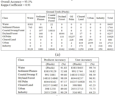
Accuracy assessment of the ISODATA classification was determined by means of a confusion matrix (sometimes called error matrix), which compares, on a class-by-class basis, the relationship between reference data (ground truth) and the corresponding results of a classification [13]. Such matrices are square, with the number of rows and columns equal to the number of classes, i.e. 11. For all classes, the numbers of reference pixels are: water (9129), coastal swamp forest (14840), dryland forest (6162), oil palm (10492), industry (350), cleared land (1250), urban (2309)and sediment plumes (1881). The diagonal elements in Table 3(a) represent the

c element at position a row and a column

c_• column sums

= =

The minimum acceptable accuracy for a class is 90% [13]. Table 3(b) shows the producer for all the classes. It is obvious that five classes possess producer accuracy higher than 90%: coastal swamp forest gives the highest (100%) and cleared land the lowest (32%). The relatively low accuracy of cleared land is mainly because 50% and 14% of its pixels were classified as urban and industry. The misclassification of cleared land pixels to the urban class is due to the fact that pixel is classified to on an image actually represents that class on the ground [13]. It is calculated by dividing each of the

diagonal elements in a confusion matrix by the total of the row in which it occurs: land (45%). A measure of overall behaviour of the ISODATA clustering can be determined by the overall accuracy, which is the total percentage of pixels correctly classified:

U respectively. The minimum acceptable overall accuracy is 85% [14]. The Kappa coefficient,

κ

is a second measure of classification accuracy which incorporates the off-diagonal elements as well as the diagonal terms to give a more robust indicating quite good agreement with the ground truth pixels.

Table 3.(a) Confusion matrix and (b) producer and user accuracy for ISODATA clustering.

(a)

B. Correlation Matrix Analysis

Classification uses the covariance of the bands; nonetheless, covariance is not intuitive; more intuitive is

correlation,

ρ

_{k ,l}, i.e. covariance normalised by the product of

the standard deviations of bands,

k

and

l

:

(

) (

)

(

k k l l

)

k,l k,l

k l k l

E I I

C − µ − µ

ρ = =

σ σ σ σ (9)

where Ck,l is the covariance between bands k and l , k and

l are the standard deviations of the measurements in bands

k

and

l

respectively,

E

is the expected value operator, and

k

I

and

I

_l and

µ

_k and

µ

_l are the intensities and means of

bands

k

and

l

respectively. When using more than two bands, it is convenient to use a correlation matrix, where the element in row

m

and column

n

that correspond to band

k

and

l

is given by _{k ,l}. If

m

=

n

, then _{k ,l}

=

1

, so this will

be the value of the diagonal elements of the matrix. Otherwise, if

m

≠

n

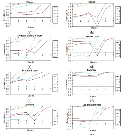
, _{k ,l} lies between -1 and 1. In order to analyse the

correlation matrices, plots of correlation versus band pair for all classes are plotted. Figure 4 shows correlation between band pairs from all identified classes, i.e. (a) water, (b) urban, (c) coastal swamp forest, (d) cleared land, (e) dryland forest, (f) industry, (g) oil palm and (h) sediment plumes. Each coloured curve represents correlation between a specific band (given by a specific colour) with all bands (on the x-axis). Landsat bands 1, 2 and 3 are located within a very close wavelength range of the visible spectrum, with their centre wavelengths differing only by about 0.1 µm. Measurements made from these bands normally exhibit similar responses and therefore are highly correlated (pink curves). Poor correlations may result from mixed pixel problem (existence of more than one class in a pixel). Correlations between lower-numbered bands (i.e. bands 1, 2 and 3) and higher-numbered bands (i.e. bands 4, 5, and 6) are much lower because involving non-adjacency wavelengths. For industry, correlation in most band pairs is quite high in ISODATA clustering due to having quite uniform surface materials, i.e. hard and bright surfaces and therefore very reflective. In other words, for industry, there are very strong relationships of variation between the brightness of pixels and mean brightness in all bands (1, 2, 3, 4, 5 and 7). For water, there is an increasing trend for the band pairs as one of the band number increases. This shows the difference of the spectral response for water when sensed from different bands; water normally has a very low reflectance in visible bands (bands 1, 2 and 3) and almost no reflectance at all in near (band 5) and mid infrared bands (band 7).

C. Mean, Standard Deviation and Decision Boundary Analysis

Despite of being very similar, both forests can still be separated quite effectively from each other using ISODATA clustering (see Figure 3). Here, we investigate further the forests in terms of mean, standard deviation and decision boundary. Figure 5(a) shows the means and (b) standard deviation of coastal swamp forest and dryland forest classes in ISODATA clustering. The means are almost the same particularly in bands 1, 2, 3 and 4, while dryland forest has a bigger mean than coastal swam forest for band 5 and 7. This shows that the means for band 5 and 7 are important in separating between the two forests. The standard deviation of coastal swamp forest is bigger than dryland forest bands 1, 2 and 3, about the same in band 4 and 7 and vice versa for band 5. Band 4 has the biggest standard deviation, indicating its ability to sense the variability within the forests, therefore is important to differentiate between plant species if further subclassification is to be made.

Figure 4. Correlations between band pairs for (a) water, (b) coastal swamp forest, (c) dryland forest, (d) oil palm, (e) urban, (f) cleared land, (g) industry

and (h) sediment plumes.

Figure 5. (a) Means of coastal swamp forest and dryland forest classes in ISODATA clustering classification. DLF and CSF are dryland forest and coastal swamp forest respectively. (b) Standard deviations of the coastal

swamp forest and dryland forest classes.

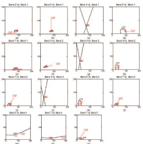
are the means for dryland forest and coastal swamp forest respectively, ‘Band k Vs. Band l’ denotes that the vertical axis is band k while horizontal axis is band l and ‘CSF’ and ‘DLF’ indicate coastal swamp forest and dryland forest respectively. The decision boundaries formed by the ISODATA clustering have the form of conic sections, i.e. pairs 2:1, 3:1 and 3:2 form an elliptic curve, pairs 5:1, 7:1, 5:2, 7:2, 5:3, 7:3, 7:5, 5:4 and 7:4 form a parabolic curve and pairs 4:1, 4:2 and 4:3 form a hyperbolic curve. Most of the regions enclosed by the boundary are owned by coastal swamp forest due to the smaller standard deviation of coastal swamp forest than dryland forest in most of the bands. It can be seen that M1 and M2 are being located within the same boundary for pairs 2:1, 3:1, 4:1, 3:2, 4:2 and 4:3 due to very small difference in mean in these bands (see Figure 5). For the rest of the pairs, i.e. 5:1, 7:1, 5:2, 7:2, 5:3, 7:3, 5:4, 7:4 and 7:5, M1 and M2 are positioned in the different sides of the boundary because it comprises of bands that seem having suitable wavelengths for the forests separation.

Figure 6. Decision boundaries between coastal swamp forest and dryland forest. ‘M1’ and ‘M2’ are the means for dryland forest and coastal swamp forest respectively. ‘Band k Vs. Band l’ denotes that the vertical axis is band k

while horizontal axis is band l and ‘CSF’ and ‘DLF’ indicate coastal swamp forest and dryland forest respectively.

VI. CONCLUSION

In this study, a detailed analysis of ISODATA clustering has been performed. ISODATA clustering classifies pixels purely based on the statistical properties of the data and does not require prior knowledge on the land cover types. The study shows that ISODATA clustering able to classify eight classes that exist in the study area with a good agreement with the reference map (overall accuracy 93% and kappa coefficient 0.91). The major drawback to ISODATA is that it misses small classes within the scene due to the highly-dependency

on the statistical properties of the data. The behaviour of the means and the standard deviations as observed in the decision space are to be the main factors that lead to the relatively good classification accuracy of ISODATA clustering.

ACKNOWLEDGMENT

The authors would like to thank the Malaysian Ministry of Higher Education (MOHE) and Universiti Teknikal Malaysia Melaka (UTeM) for funding this study, and the Malaysian Remote Sensing Agency for providing the data (ARSM).

REFERENCES

[1] C. P. Low and J. Choi (2004), A hybrid approach to urban land use/cover mapping using Landsat 7 Enhanced Thematic Mapper Plus (ETM+) images, International Journal of Remote Sensing, 25, 2687 – 2700.

[2] Z. Wang, J.R. Jensen and I.M. Jungho (2010), An automatic region-based image segmentation algorithm for remote sensing applications,

Environmental Modelling & Software, 25, 1149 – 1165.

[3] Z. Xia, S. Rui, Z. Bing, and T. Qingxi (2008), Land cover classification of the North China Plain using MODIS EVI time series, ISPRS Journal of Photogrammetry and Remote Sensing, 63, 476 – 484, 2008.

[4] M.H. Ismail and K. Jusoff (2008), Satellite data classification accuracy assessment based from reference dataset, International Journal of Computer and Information Science and Engineering, 2, 96 – 102.

[5] S.M. Baban and K.W. Yusof (2001), Mapping land use/cover distribution on a mountainous tropical island using remote sensing and GIS, International Journal of Remote Sensing, 22, 1909 – 1918.

[6] N.M. Yusoff (2005), RazakSAT - Technology advent in high resolution imaging system for small satellite, Proceedings of the 26th ACRS (Asian Conference on Remote Sensing) Hanoi, Vietnam, Nov. 7-11, 2005, AARS, Hanoi.

[7] D. M. Memarsadeghi, D.M. Mount, N. S. Netanyahu, and J. Le Moigne (2007), A Fast implementation of the ISODATA clustering algorithm,

International Journal of Computational Geometry and Applications, 17, 71 – 103.

[8] J.R. Jensen (1996), Introductory Digital Image Processing: A Remote Sensing Perspective, Pearson Prentice Hall, New Jersey, USA.

[9] B.L. Markham, J.C. Storey, D.L. Williams. and J.R. Irons (2004), Landsat sensor performance: history and current status, IEEE Transaction on Geoscience and Remote Sensing, 42, 2691 – 2694.

[10] G. Chander, B.L. Markham and D.L. Helder (2009), Summary of current radiometric calibration coefficients for Landsat MSS, TM, ETM+ and EO-1 ALI sensors, Remote Sensing of Environment, 133, 893 – 903.

[11] A. Ahmad, M. Hashim, M.N. Hashim, M.N. Ayof, and A.S. Budi, “The Use of Remote Sensing and GIS to Estimate Air Quality Index (AQI) Over Peninsular Malaysia,” GIS development, 2006, p. 5pp.

[12] A. Ahmad, and S. Quegan (2012), Cloud masking for remotely sensed data using spectral and principal components analysis, Engineering, Technology & Applied Science Research (ETASR), 2, 221 – 225.

[13] M. Story and R. Congalton (1986), Accuracy assessment: a user's perspective, Photogrammetric Engineering and Remote Sensing, 52, 397 – 399.