Classification Simulation of RazakSAT Satellite.

(1)

Procedia Engineering 53 ( 2013 ) 472 – 482

Selection and peer-review under responsibility of the Research Management & Innovation Centre, Universiti Malaysia Perlis doi: 10.1016/j.proeng.2013.02.061

Malaysian Technical Universities Conference on Engineering & Technology 2012, MUCET 2012

Part 3 - Civil and Chemical Engineering

Classification Simulation of RazakSAT Satellite

Asmala Ahmad

a,

*

ªCenter of Advanced Computing Technologies (C-ACT) Faculty of Information and Communication Technology

Universiti Teknikal Malaysia Melaka (UTeM) Hang Tuah Jaya, Melaka, Malaysia

Abstract

This study presents simulation of land cover classification for RazakSAT satellite. The simulation makes use of the spectral capability of Landsat 5 TM satellite that has overlapping bands with RazakSAT. The classification is performed using Maximum Likelihood (ML), a supervised classification method that is based on the Bayes theorem. ML makes use of a discriminant function to assign pixel to the class with the highest likelihood. Class mean vector and covariance matrix are the key inputs to the function and are estimated from the training pixels of a particular class. The accuracy of the classification for the simulated RazakSAT data is accessed by means of a confusion matrix. The results show that RazakSAT tends to have lower overall and individual class accuracies than Landsat mainly due to the unavailability of mid-infrared bands that hinders separation between different plant types.

Selection and/or peer-review under responsibility of the Research Management & Innovation Centre, Universiti Malaysia Perlis.

Keywords: RazakSAT, Maximum Likelihood, Accuracy

1.Introduction

The Malaysian second remote sensing satellite, RazakSAT (Figure 1), is named after the Malaysian second prime minister - the late Abdul Razak, also known as the father of Malaysian Development. It was successfully launched into orbit by a Falcon 1 rocket on July 14, 2009, aiming to serve Malaysia with remote sensing data for applications mainly in agriculture, landscape mapping, forestry and urban planning.

(a) (b)

Fig.1. (a) RazakSAT satellite (Malaysian National Space Agency 2007) and (b) RazakSAT Near Equatorial Orbit (NEqO) [12].

As it is meant to serve the interest of Malaysia and other countries (Table 1) in the near-Equatorial belt, the satellite was

(2)

launched into a Near Equatorial Orbit (NEqO) with inclination 9°, to take advantage of the corresponding opportunities to gather images at 14 times daily and overcome the major obstacle for passive remote sensing, cloud cover [11].

Table 1. List Of Countries Covered By Neqo At 9o

Inclination [11]

Continent Countries

Asia India, Indonesia, Malaysia, Maldives, Philippines, Sri Lanka, Thailand

Africa

Angola, Benin, Burundi, Cameroon, Central African Republic, Chad, Cote d'Ivoire, Ethiopia, Gabon, Guinea, Kenya, Liberia, Nigeria, Rwanda, Sierra Leone, Somalia, Sudan, Tanzania, Uganda, Zaire

Latin America

Brazil, Colombia, Ecuador, French Guiana, Guyana, Panama, Peru, Surinam, Venezuela

The RazakSAT satellite carries a medium-sized aperture camera (MAC) to be used as an earth observation payload. It is a push-broom type high resolution camera with one panchromatic and four multispectral bands. The panchromatic band with 2.5 m ground sampling resolution operates at 0.510 to 0.730 m wavelength. The other four bands operate at 0.450 to 0.520 m (blue), 0.520 to 0.600 m (green), 0.630 to 0.690 m (red) and 0.760 to 0.890 m (near infrared) wavelength respectively (Table 2). Unfortunately, due to unknown circumstances, the RazakSAT data is still available for users, although nearly after three and a half year since its launch.

Table 2. Razaksat Specifications [13]

Parameter Descripion Altitude 685 km (nominal) Inclination 9º

Spectral channels 5 visible and 1 panchromatic bands: Band 1: 0.450 0.520 m (Blue) Band 2: 0.520 0.600 m (Green) Band 3: 0.630 0.690 m (Red) Band 4: 0.760 0.890 m (Near infrared) Band 5: 0.510 0.730 m (Panchromatic) Ground Sampling 5.0 m (visible)

2.5 (panchromatic) Designed Mission Lifetime > 3 years

One of the most common remote sensing satellites is Landsat, initiated by NASA (National Aeronautical and Space Administration) in 1972 [3]. The Landsat satellites have been providing optical data for almost 40 years. Landsat 1 3 launched in the 1970s and used Multispectral Scanner (MSS), while Landsat 4 5, launched in the 1980s, use Thematic Mapper (TM) as their main sensor. The latest Landsat 7, launched in 1999, uses the Enhanced Thematic Mapper (ETM+). Comparison between the specifications of these satellites is given in Table 3. Landsat 5 was launched on March 1, 1984 with an expected lifetime of 5 years, and, after more than 27 years of operation, has provided the global science community with over 900,000 individual scenes and is the longest running satellite of the series (Figure 2).

(3)

Table 3. Landsat 5 Tm Satellite Specifications [3]

Parameter Description

Spectral Bands 4 VNIR, 2 SWIR, 1 thermal Spatial Resolution

(IFOV)

30 m VNIR, SWIR 120 m thermal Sampling 1 samples/IFOV along scan Cross Track

Coverage 185 km Radiometric

Resolution 8 bits Radiometric

Calibration Internal lamps, shutter and black body Scanning Mechanism Bidirectional Scanning with Scan Line

Corrector

Equatorial Crossing 9:45 AM +/- 15 minutes Type Sun synchronous, near polar Inclination 98.2°

Landsat 5 TM level 1 data come in Product Generation System (LPGS) format and need to be converted into a physically meaningful common radiometric unit, representing the at-sensor spectral radiance. The Level 1 Landsat 5 TM data received by users are in scaled 8-bit numbers, Q_cal, or also known as digital number (DN). Conversion from Q_cal to spectral radiance, L , can be done by using [5]:

where, L is the spectral radiance at the sensor's aperture (W/ m2 , Q_cal is the quantized calibrated pixel value (DN), cal min

Q is the minimum quantised calibrated pixel value corresponding to L_min (DN), Q_{cal max} is the maximum quantised calibrated pixel value corresponding to L_max (DN), L_min is the spectral at-sensor radiance that is scaled to Q_{cal min} (W/ m2 L_max is the spectral at-sensor radiance that is scaled to Q_{cal max} (W/ m2 Q_{cal min} and Q_{cal max} are 1 and 255 respectively.

Table 4 showsL_min , L_max and the mean exoatmospheric solar irradiance (E ).

Table 4. Landsat Tm Spectral Range, Post-Calibration Dynamic Ranges And The Mean Exoatmospheric Solar Irradiance [5]

Band Spectral range Centre

wavelength Lmin Lmax E

Scene-to-scene variability can be reduced by converting the at-sensor spectral radiance to top-of-atmosphere (TOA) reflectance, also known as in-band planetary albedo. By performing this conversion, the cosine effect of different solar zenith angles due to the time difference between data acquisitions is removed, different values of the exoatmospheric solar irradiance arising from spectral band differences are compensated and the variation in the Earth Sun distance between different data acquisition dates is corrected. The TOA reflectance can be computed by using [5]:

(4)

Where, L

is the spectral radiance at the sensor's aperture (W m-2 sr-1 -1), d is the Earth Sun distance (astronomical units), E is the mean exoatmospheric solar irradiance (W m-2 -1) and _s is the solar zenith angle (degrees). d can be generated from the Jet Propulsion Laboratory (JPL) Ephemeris at http://ssd.jpl.nasa.gov/?horizons or can be obtained from the literature (e.g.[5]). Conversion to at-sensor spectral radiance and TOA reflectance can be performed by using built-in tools in high-end image processing software, such as ENVI.

This study attempts to simulate the RazakSAT land cover classification by making use of the Landsat data. The classification is carried out by means of Maximum Likelihood method.

2.Maximum Likelihood (ML) Classification

ML is a supervised classification method derived from the Bayes theorem, which states that the a posteriori distribution P(i| ), i.e., the probability that a pixel with feature vector belongs to class i, is given by:

P i P i

P i |

P (3)

where,P i is the likelihood function, P i is the a priori information, i.e., the probability that class i occurs in the study

area and P is the probability that is observed, which can be written as:

M i 1

P P | i P i (4)

where, M is the number of classes. P is often treated as a normalisation constant to ensure M i 1

P i | sums to 1. Pixel

x is assigned to class i by the rule:

x i if P i | P j | (5)

ML often assumes that the distribution of the data within a given class i obeys a multivariate Gaussian distribution. It is then convenient to define the log likelihood (or discriminant function):

t 1

Since log is a monotonic function, Equation (3) is equivalent to:

x i if g ( )_i g ( )_j (7)

Each pixel is assigned to the class with the highest likelihood or labelled as unclassified if the probability values are all below a threshold set by the user [7]. The general procedures in ML are as follows:

1. The number of land cover types within the study area is determined.

(5)

ij

J 2 1 e (8)

where, is the Bhattacharyya distance and is given by [7]:

i j

Jij ranges from 0 to 2.0, where Jij > 1.9 indicates good separability of classes, moderate separability for 1.0 Jij 1.9 and poor separability for Jij < 1.0.

3. The training pixels are then used to estimate the mean vector and covariance matrix of each class.

4. Finally, every pixel in the image is classified into one of the desired land cover types or labeled as unknown.

In ML classification, each class is enclosed in a region in multispectral space where its discriminant function is larger than that of all other classes. These class regions are separated by decision boundaries, where, the decision boundary between class i and j occurs when:

i j

g ( ) g ( ) (10)

For multivariate normal distributions, this becomes:

t 1

This is a quadratic function in N dimensions. Hence, if we consider only two classes, the decision boundaries are conic sections (i.e. parabolas, circles, ellipses or hyperbolas).

3.ML Using Landsat Data

The study area was located in Selangor, Malaysia, covering approximately 840 km2 within longitude 101

101 latitude 2 -5 TM dated

(6)

Malaysian Remote Sensing Agency. 11 main classes identified were water, coastal swamp forest, dryland forest, oil palm, rubber, industry, cleared land, urban, sediment plumes, coconut and bare land.

Fig. 3. The study area from (a) the land cover map and (b) the Landsat-5 TM with bands 5 4 and 3 assigned to the red, green and blue channels. Cloud and its shadow are masked in black.

Training areas were established by choosing one or more polygons for each class. In order to select a good training area for a class, the important properties taken into consideration are its uniformity and how well they represent the same class throughout the whole image [8]. Class separability of the chosen training pixels (extracted from the training area) was determined by means of the JM distance. Fifty pairs have JM distance between 1.9 and 2.0 indicating good separability, four from 1.0 to 1.9 indicating moderate separability and one less than 1.0 indicating poor separability. The worst separability, possessed by the urban industry pair (0.947), was expected since both have very similar spectral characteristics. For each class, these training pixels provide values from which to estimate the mean and covariances of the spectral bands used.

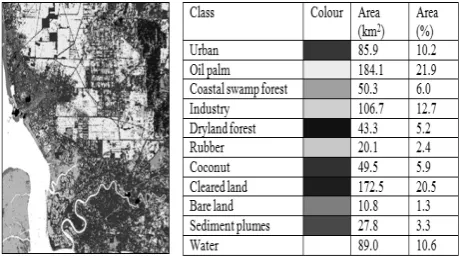
The outcome of ML classification after assigning the classes with suitable colours, is shown in Figure 4: coastal swamp forest (green), dryland forest (blue), oil palm (yellow), rubber (cyan), cleared land (purple), coconut (maroon), bare land (orange), urban (red), industry (grey), sediment plumes (sea green) and water (white). Clouds and their shadows are masked black. The areas in terms of percentage and square kilometres were also computed; the classes with the largest area are oil palm, cleared land and industry. Although being similar, coastal swamp forest and dryland forest can be clearly seen in the south-west and north-east of the classified image, as indicated by the reference map. Coastal swamp forest covers most of the Island and coastal regions in the south-west of the scene. Most of the dryland forest can be recognised as a large straight-edged region in the north-east. Oil palm and urban dominate the northern and southern parts respectively. Rubber appears as scattered patches that mostly are surrounded by oil palms. Industry can be recognised as patches near the urban areas, especially in the south-west and north-east. Coconut can be seen in the coastal area in the north-west of the image. A quite large area of bare land can be seen in the east, while cleared land can be seen mostly in the north, south and south-east of the image.

Fig. 4. ML classification using band 1, 2, 3, 4, 5 and 7 of Landsat TM and the class areas in terms of square kilometre and percentage

(7)

coconut (159), bare land (313) and sediment plumes (1881). The diagonal elements in Table 5 represent the pixels of correctly assigned pixels and are also known as the producer accuracy.Producer accuracy is a measure of the accuracy of a particular classification scheme and shows the percentage of a particular ground class that is correctly classified. It is calculated by dividing each of the diagonal elements in Table 5 by the total of each column respectively:

(13)

where,

th th

aa

a

c element at position a row and a column

c column sums

The minimum acceptable accuracy for a class is 90% [10]. It is obvious that all classes possess producer accuracy higher than 90%: bare land gives the highest (100%) and oil palm the lowest (92.4%). The relatively low accuracy of oil palm is mainly because 6% and 1% of its pixels were classified as coconut and cleared land. The misclassification of oil palm pixels to the coconut class is due to the fact that oil palm and coconut have a similar physical structure, so tend to have similar spectral behavior and therefore can easily be misclassified as each other. User Accuracy is a measure of how well the classification is performed. It indicates the percentage of probability that the class which a pixel is classified to on an image actually represents that class on the ground [10]. It is calculated by dividing each of the diagonal elements in a confusion matrix by the total of the row in which it occurs:

ii

c row sum. Coastal swamp forest, dryland forest, oil palm, sediment plumes, water, bare land and urban show a user accuracy of more than 90%. Rubber, cleared land and industry possess accuracy between 70% and 90%, while the worst accuracy is possessed by coconut (16%). The low accuracy of coconut is because the oil palm pixels tend to be classified as coconut because they having similar spectral properties to oil palm. A measure of overall behaviour of the ML classification can be determined by the overall accuracy, which is the total percentage of pixels correctly classified:

U

where, Q and U is the total number of pixels and classes respectively. The minimum acceptable overall accuracy is 85% [6]. The Kappa coefficient, is a second measure of classification accuracy which incorporates the off-diagonal elements as well as the diagonal terms to give a more robust assessment of accuracy than overall accuracy. It is computed as [9]:

U U

where, c_a row sums. The ML classification yielded an overall accuracy of 97.4% and kappa coefficient 0.97, indicating very high agreement with the ground truth.

aa

a

c

(8)

Table 5. Confusion Matrix For Ml Classification Using Landsat Data

4.ML Using Simulated RAZKSAT Data

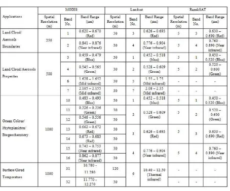
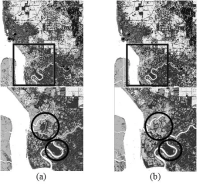
Table 6 shows relationship between Landsat and RazakSAT satellite. For comparison, some of MODIS bands are also shown. Compared to Landsat, RazakSAT only has 4 multispectral bands and does not measure in mid-infrared wavelengths. Here, ML classification using bands 1, 2, 3 and 4 of Landsat dataset (i.e. correspond to bands 1, 2, 3 and 4 of RazakSAT) was performed in order to simulate RazakSAT classification. The labelling and colour scheme in Figure 4 were used. Figure 5 is the ML classification using (a) Landsat bands 1, 2, 3 and 4 and (b) same as shown in Figure 4, but is shown again for convenient. The bottom images are the enlarged versions of the region in the blue box in the top images. The circles indicate areas where apparent misclassification occurred; i.e. cleared land pixels (bottom circle) and industry pixels (top circle) being misclassified as urban.

Table 6. Relationship Between Modis, Landsat And Razaksat Satellite

(9)

Fig. 5. ML classification of the study area in Selangor, Malaysia using (a) bands 1, 2, 3 and 4 (top), (b) bands 1, 2, 3, 4, 5 and 7 (top) and enlarged versions of the area in the blue box (bottom). The Circles indicate areas where apparent misclassification occurred.

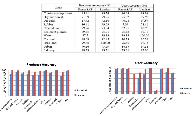
Table 8 shows the producer and user accuracy of simulated RazakSAT data for all classes; those of Landsat is also given for comparison. To better visualise the difference, plots of producer and user accuracy for the simulated RazakSAT and Landsat data are given in Figure 6. The highest producer accuracy is possessed by bare land, industry and water, while urban, cleared land and sediment plumes have the worst accuracy. For user accuracy, water, bare land and coastal swamp forest have the highest accuracy while rubber, coconut and cleared land have the lowest accuracy.

The lower user accuracies of rubber, coconut and cleared land indicates high commission error for these classes, meaning that there is a probability (proportionate to the error) that pixel classified as rubber, coconut and cleared land may not actually exist on the ground. On the other hand, urban, cleared land and sediment plumes have the worst producer accuracy due to the high omission error, meaning that there is a probability (proportionate to the errors) that the pixels for these classes were classified incorrectly. The maximum wavelength that RazakSAT can sense is about 0.9 m, while that of Landsat is 2.35 m. Wavelengths beyond 1.3 m, e.g. 1.4 m and 1.9 m are known as water absorption bands are useful to differentiate between land and water boundary as well as between different plant types. The water in the leaf absorbs strongly at these wavelength. Clearly, these wavelengths are useful to differentiate plants due to the different amount of water stored in different plant leaves. This leads to the smaller producer and user accuracy of the simulated RazakSAT data compared to the Landsat data in most plant classes. It can be seen that non plant classes, i.e. urban and cleared land, are also affected due to normally having minimal amount vegetation and surfaces with different moisture content. As expected the least difference is shown by industry and bare land due to having almost no vegetation and covered with uniform reflective surfaces.

This shows that when only considering the spectral capability of the bands, RazakSAT tends to produce classification with lower accuracy than Landsat. However, RazakSAT bands have a higher spatial resolution (5 m) than Landsat (30 m) and is equipped with a panchromatic band (2.5 m spatial resolution), which may be able to increase the classification accuracy.

(10)

Table 8. Producer And User Accuracy Of Classification Using Simulated Razaksat And Landsat Data

Fig. 6. Plots of producer (top) and user (bottom) accuracy for simulated RazakSAT and Landsat data

5.Conclusion

The study presented here makes use of the moderate resolution Landsat 5 TM data to simulate the performance of RazakSAT classification. The unavailability of RazakSAT data allows limited analysis to anticipate its actual performance. The simulation of RazakSAT classification analysis using Landsat data shows that although without the mid-infrared bands, RazakSAT is still able to classify the study area with accuracy only slightly lower than Landsat. It is undeniable that the main shortcoming of RazakSAT is the unavailability of mid-infrared bands that hampers its capability to distinguish between vegetations and surfaces. Nonetheless, the availability of a panchromatic band and the higher spatial resolution of the multispectral bands confer major advantages of RazakSAT compared to the Landsat.

Acknowledgement

The author would like to thank the Malaysian Ministry of Higher Education (MOHE) and Universiti Teknikal Malaysia Melaka (UTeM) for funding this study and the Malaysian Remote Sensing Agency (ARSM), Ministry of Science, Technology and Innovation (MOSTI) for providing the data.

References

[1] A. Ahmad, and S. Quegan (2012), Cloud masking for remotely sensed data using spectral and principal components analysis, Engineering, Technology & Applied Science Research (ETASR), 2, 221 225.

[2] A. Ahmad, M.N. Ayof, S.B. Agus, H. Sakidin, and S.S.S. Ahmad (2006), Smoke detection using remote sensing technique. Prosiding Seminar Pencapaian Penyelidikan KUTKM 2006 (REACH 06). 284-293.

[3] B.L. Markham, J.C. Storey, D.L. Williams. and J.R. Irons (2004), Landsat sensor performance: history and current status, IEEE Transaction on Geoscience and Remote Sensing, 42, 2691 2694.

[4] ENVI (2006), , Research Systems Inc., USA.

[5] G. Chander, B.L. Markham and D.L. Helder (2009), Summary of current radiometric calibration coefficients for Landsat MSS, TM, ETM+ and EO-1 ALI sensors, Remote Sensing of Environment, 133, 893 903.

(11)

[7] J.A. Richards 1999, Remote sensing digital image analysis: An introduction. Springer-Verlag, Berlin, Germany.

[8] J.B. Campbell 2002, Introduction to remote sensing, Taylor & Francis, London.

[9] J.R. Jensen (1996), Introductory Digital Image Processing: A Remote Sensing Perspective, Pearson Prentice Hall, New Jersey, USA.

[10] M. Story and R. Congalton (1986), Accuracy assessment: a user's perspective, Photogrammetric Engineering and Remote Sensing, 52, 397 399.

[11] N.M. Yusoff (2005), RazakSAT - Technology advent in high resolution imaging system for small satellite, Proceedings of the 26th ACRS (Asian Conference on Remote Sensing)Hanoi, Vietnam, Nov. 7-11, 2005, AARS, Hanoi.

[12] N.M. Yusoff, S.A. Ahmad and M. Othman (2002), Utilization of TiungSAT-1 data for environmental assessment and monitoring, Canadian International Development Agency (CIDA)-Canadian Space Agency (CSA) Conference, Space Applications for Sustainable Development, Hull, Canada, May 21-22, 2002, CIDA-CSA, Canada.

[13] N. S. Wai, A. A.Tan, J. W. S. Mee, Ismail, M. & M.D. Subari, (2009). Proceedings of International Conference on Recent Advances in Space Technologies, 2009 (RAST '09), 277 282.

[14] S.A. Ackerman, K.I. Strabala, W.P. Menzel, R.A. Frey, C.C. Moeller and L.E. Gumley (1998), Discriminating clear-sky from clouds with MODIS, Journal of Geophysical Research, 103, 32141 32157.

[15] T.M. Lillesand, R.W. Kiefer and J.W. Chipman (2004), Remote Sensing and Image Interpretation, John Wiley & Sons, Hoboken, NJ, USA.