Applied Mathematical Sciences, Vol. 6, 2012, no. 129, 6425 - 6436
Analysis of Maximum Likelihood Classification
on Multispectral Data
Asmala Ahmad
Department of Industrial Computing
Faculty of Information and Communication Technology Universiti Teknikal Malaysia Melaka
Hang Tuah Jaya, 76100 Durian Tunggal, Melaka, Malaysia [email protected]
Shaun Quegan
School of Mathematics and Statistics University of Sheffield
Sheffield, United Kingdom
Abstract
The aim of this paper is to carry out analysis of Maximum Likelihood (ML) classification on multispectral data by means of qualitative and quantitative approaches. ML is a supervised classification method which is based on the Bayes theorem. It makes use of a discriminant function to assign pixel to the class with the highest likelihood. Class mean vector and covariance matrix are the key inputs to the function and can be estimated from the training pixels of a particular class. In this study, we used ML to classify a diverse tropical land covers recorded from Landsat 5 TM satellite. The classification is carefully examined using visual analysis, classification accuracy, band correlation and decision boundary. The results show that the separation between mean of the classes in the decision space is to be the main factor that leads to the high classification accuracy of ML.
1 Introduction
Maximum Likelihood (ML) is a supervised classification method derived from the Bayes theorem, which states that the a posteriori distribution P(i|ω), i.e., the probability that a pixel with feature vector ω belongs to class i, is given by:
( ) ( ) ( )
ω|( )
ωω
P i P i P |
i
P = (1)
where P(ω|i) is the likelihood function, P(i) is the a priori information, i.e., the probability that class i occurs in the study area and P
( )
ω is the probability that ω is observed, which can be written as:( )
P( ) ( )
|i P iP
M
1 i
∑
= = ωω (2)
where M is the number of classes. P
( )
ω is often treated as a normalisationconstant to ensure
∑
( )
=
M
1 i
| i
P ω sums to 1. Pixel x is assigned to class i by the rule:
x∈i if P(i|ω) > P(j|ω) for all j≠i (3)
ML often assumes that the distribution of the data within a given class i obeys a multivariate Gaussian distribution. It is then convenient to define the log likelihood (or discriminant function):
( )
(
) (
)
( )
( )
i 1i t
i ln C
2 1
π
2 ln 2 N C
2 1 i P ln ) (
g ω = ω| =− ω−μi − ω−μi − − (4)
Since log is a monotonic function, Equation (3) is equivalent to:
x∈i if gi(ω) > gj(ω) for all j≠i . (5)
Each pixel is assigned to the class with the highest likelihood or labelled as unclassified if the probability values are all below a threshold set by the user [9]. The general procedures in ML are as follows:
1. The number of land cover types within the study area is determined.
For normally distributed classes, the JM separability measure for two classes, Jij, is
defined as follows [4]:
(
α)
ij 21 e
J = − − (6)
where α is the Bhattacharyya distance and is given by [4]:
(
) (
) ( )
i j 1
t i j
i j
C C
C C 2
1 1
α ln
8 2 2 C C
− ⎛⎜ + ⎞⎟ ⎡ + ⎤ ⎜ ⎟ ⎢ ⎥ = − − + ⎜ ⎟ ⎢ ⎥ ⎣ ⎦ ⎜⎜ ⎟⎟ ⎝ ⎠
i j i j
μ μ μ μ (7)
Jij ranges from 0 to 2.0, where Jij > 1.9 indicates good separability of classes,
moderate separability for 1.0 ≤ Jij ≤1.9 and poor separability for Jij < 1.0 [2].
3. The training pixels are then used to estimate the mean vector and covariance matrix of each class.
4. Finally, every pixel in the image is classified into one of the desired land cover types or labelled as unknown.
In ML classification, each class is enclosed in a region in multispectral space where its discriminant function is larger than that of all other classes. These class regions are separated by decision boundaries, where, the decision boundary between class i and j occurs when:
gi(ω) = gj(ω) (8)
For multivariate normal distributions, this becomes:
(
) (
)
( )
( )
(
) (
)
( )
ln( )
C 0 2 1 π 2 ln 2 N C 2 1 C ln 2 1 π 2 ln 2 N C 2 1 j 1 j t i 1 i t = ⎟ ⎠ ⎞ ⎜ ⎝ ⎛− − − − − − − − − − − − − j j i i μ ω μ ω μ ω μ ω (9)which can be written as:
(
−) (
tC11 −)
−ln( )
Ci +(
−) (
tCj1 −)
+ln( )
Cj =0− − −
j j
i
i ω μ ω μ ω μ
μ
ω (10)
2 Methodology
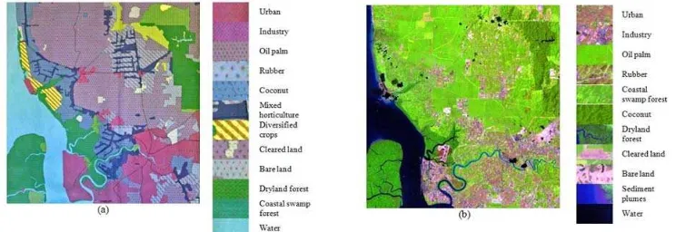
The study area was located in Selangor, Malaysia, covering approximately 840 km2 within longitude 101° 10’ E to 101°30’ E and latitude 2°99’ N to 3°15’ N (Figure 1). The satellite data come from bands 1 (0.45 – 0.52 µm), 2 (0.52 – 0.60 µm), 3 (0.63 – 0.69 µm), 4 (0.76 – 0.90 µm), 5 (1.55 – 1.75 µm) and 7 (2.08 – 2.35 µm) of Landsat-5 TM dated 11th February 1999. The satellite records surface reflectance with 30 m spatial resolution from a height of 705 km. Prior to any data processing, masking of cloud and its shadow were carried out based on threshold approach [8], [1]. Visual interpretation of the Landsat data (Figure 1(b)) was carried out to identify main land covers within the study area. The task was aided by a reference map (Figure 1(a)), produced in October 1991 by the Malaysian Surveying Department and Malaysian Remote Sensing Agency using ground surveying and SPOT satellite data. 11 main classes were identified, i.e. water, coastal swamp forest, dryland forest, oil palm, rubber, industry, cleared land, urban, sediment plumes, coconut and bare land.
Fig. 1. The study area from (a) the land cover map and (b) the Landsat-5 TM with bands 5 4 and 3 assigned to the red, green and blue channels. Cloud and
its shadow are masked in black.
3 Analysis of ML classification
3.1 Visual Analysis
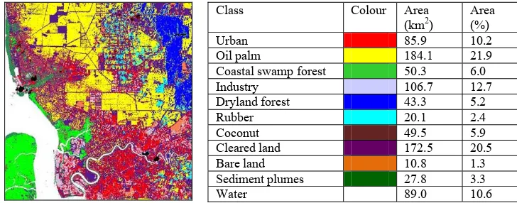
The outcome of ML classification after assigning the classes with suitable colours, is shown in Figure 2: coastal swamp forest (green), dryland forest (blue), oil palm (yellow), rubber (cyan), cleared land (purple), coconut (maroon), bare land (orange), urban (red), industry (grey), sediment plumes (sea green) and water (white). Clouds and their shadows are masked black. The areas in terms of percentage and square kilometres were also computed; the classes with the largest area are oil palm, cleared land and industry. Although being similar, coastal swamp forest and dryland forest can be clearly seen in the south-west and north-east of the classified image, as indicated by the reference map. Coastal swamp forest covers most of the Island and coastal regions in the south-west of the scene. Most of the dryland forest can be recognised as a large straight-edged region in the north-east. Oil palm and urban dominate the northern and southern parts respectively. Rubber appears as scattered patches that mostly are surrounded by oil palms. Industry can be recognised as patches near the urban areas, especially in the south-west and north-east. Coconut can be seen in the coastal area in the north-west of the image. A quite large area of bare land can be seen in the east, while cleared land can be seen mostly in the north, south and south-east of the image.
Class Colour Area
(km2)
Area (%)
Urban 85.9 10.2
Oil palm 184.1 21.9
Coastal swamp forest 50.3 6.0
Industry 106.7 12.7
Dryland forest 43.3 5.2
Rubber 20.1 2.4
Coconut 49.5 5.9
Cleared land 172.5 20.5
Bare land 10.8 1.3
Sediment plumes 27.8 3.3
Water 89.0 10.6
Fig. 2. ML classification using band 1, 2, 3, 4, 5 and 7 of Landsat TM and the class areas in terms of square kilometre and percentage.
3.2 Accuracy Analysis
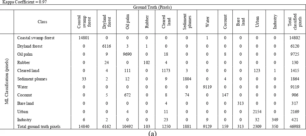
classes, the numbers of reference pixels are: rubber (103), water (9129), coastal swamp forest (14840), dryland forest (6162), oil palm (10492), industry (350), cleared land (1250), urban (2309), coconut (159), bare land (313) and sediment plumes (1881). The diagonal elements in Table 1(a) represent the pixels of correctly assigned pixels and are also known as the producer accuracy.Producer accuracy is a measure of the accuracy of a particular classification scheme and shows the percentage of a particular ground class that is correctly classified. It is calculated by dividing each of the diagonal elements in Table 1 (a) by the total of each column respectively:
aa a
c
Producer accuracy 100 %
c•
= × (11)
where,
th th
aa a
c element at position a row and a column c• column sums
= =
The minimum acceptable accuracy for a class is 90% [7]. Table 1(b) shows the producer for all the classes. It is obvious that all classes possess producer accuracy higher than 90%: bare land gives the highest (100%) and oil palm the lowest (92.4%). The relatively low accuracy of oil palm is mainly because 6% and 1% of its pixels were classified as coconut and cleared land. The misclassification of oil palm pixels to the coconut class is due to the fact that oil palm and coconut have a similar physical structure, so tend to have similar spectral behaviour and therefore can easily be misclassified as each other. User Accuracy is a measure of how well the classification is performed. It indicates the percentage of probability that the class which a pixel is classified to on an image actually represents that class on the ground [7]. It is calculated by dividing each of the diagonal elements in a confusion matrix by the total of the row in which it occurs:
ii i
c
User accuracy 100 %
c•
= × (12)
U aa a 1
c
Overall accuracy 100 % Q
=
=
∑
× (13)where, Q and U is the total number of pixels and classes respectively. The minimum acceptable overall accuracy is 85% [3]. The Kappa coefficient, κ is a second measure of classification accuracy which incorporates the off-diagonal elements as well as the diagonal terms to give a more robust assessment of accuracy than overall accuracy. It is computed as [6]:
U U
aa a a 2 a 1 a 1
U a a
2 a 1
c c c
Q Q c c 1 Q • • = = • • = − κ = −
∑
∑
∑
… (14)where ca• = row sums. The ML classification yielded an overall accuracy of 97.4% and kappa coefficient 0.97, indicating very high agreement with the ground truth.
Table 1: Confusion Matrix for ML Classification.
Overall Accuracy = 97.4% Kappa Coefficient = 0.97
Ground Truth (Pixels)
Class Coa st al sw am p fore st D ryl an d fore st O il p al m Ru bbe r Cl ea re d la nd S edi m ent pl um es W at er Co co nut Ba re la nd U rba n In dus tr y T o ta l cl as si fi ed pi xe ls M L Cl as si fi ca ti o n (pi x el s)
Coastal swamp forest 14801 0 0 0 0 0 1 0 0 0 0 14802 Dryland forest 0 6116 3 1 0 0 0 0 0 0 0 6120 Oil palm 0 9 9690 0 18 0 0 8 0 0 0 9725
Rubber 0 24 0 102 4 0 0 0 0 0 0 130
Cleared land 0 4 111 0 1173 3 0 0 0 123 1 1415 Sediment plumes 33 2 12 0 9 1804 0 4 0 0 0 1864
Water 0 0 0 0 0 0 9119 0 0 0 0 9119
Coconut 0 5 672 0 8 74 0 147 0 0 0 906
Bare land 0 0 0 0 4 0 0 0 313 0 0 317
Urban 0 0 4 0 11 0 0 0 0 2154 0 2169
Industry 6 2 0 0 23 0 9 0 0 32 349 421
Total ground truth pixels 14840 6162 10492 103 1250 1881 9129 159 313 2309 350 46988
Class Producer Accuracy User Accuracy
(Pixels) (%) (Pixels) (%) Coastal swamp forest 14801/14840 99.74 14801/14802 99.99
Dryland forest 6116/6162 99.25 6116/6120 99.93 Oil palm 9690/10492 92.36 9690/9725 99.64
Rubber 102/103 99.03 102/130 78.46 Cleared land 1173/1250 93.84 1173/1415 82.90
Sediment plumes 1804/1881 95.91 1804/1864 96.78
Water 9119/9129 99.89 9119/9119 100.00 Coconut 147/159 92.45 147/906 16.23 Bare land 313/313 100.00 313/317 98.74
Urban 2154/2309 93.29 2154/2169 99.31 Industry 349/350 99.71 349/421 82.90
(b)
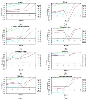
3.3 Correlation Matrix Analysis
Classification uses the covariance of the bands; nonetheless, covariance is not intuitive; more intuitive is correlation, ρk,l, i.e. covariance normalised by the product of the standard deviations of bands, k and l :
(
) (
)
(
k k l l)
k,l k,l
k l k l
E I I
C −μ −μ
ρ = =
σ σ σ σ (15)
(existence of more than one class in a pixel). Correlations between lower-numbered bands (i.e. bands 1, 2 and 3) and higher-lower-numbered bands (i.e. bands 4, 5, and 6) are much lower because involving non-adjacency wavelengths. From Figure 3, for cleared land and sediment plumes, correlation in most band pairs is quite high in ML, especially for bands 1, 2 and 3, which corresponds to the higher accuracy in these classes in ML. For certain classes, such as water (with very low reflectances), the superiority of ML is even clearer, as shown not only by the correlations from bands 1, 2 and 3, but also 4, 5 and 7 in ML that have high correlations. A high correlation is shown by industry (with very high reflectances) due to the strong relationships of variation between the brightness of pixels and mean brightness in all bands (1, 2, 3, 4, 5 and 7).
Fig. 3. Correlations between band pairs for (a) water, (b) coastal swamp forest, (c) dryland forest, (d) oil palm, (e) urban, (f) cleared land, (g) industry and (h)
sediment plumes.
3.4 Mean, Standard Deviation and Decision Boundary Analysis
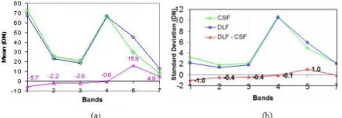
mean, standard deviation and decision boundary. Figure 4(a) shows the means and (b) standard deviation of coastal swamp forest and dryland forest classes in ML. The means are almost the same particularly in bands 1, 2 and 3. The standard deviation of coastal swamp forest is bigger than dryland forest in most of the bands, except band 5.
Fig. 4. (a) Means of coastal swamp forest and dryland forest classes in ML classification. DLF and CSF are dryland forest and coastal swamp forest respectively. (b) Standard deviations of the coastal swamp forest and dryland
forest classes in ML classification
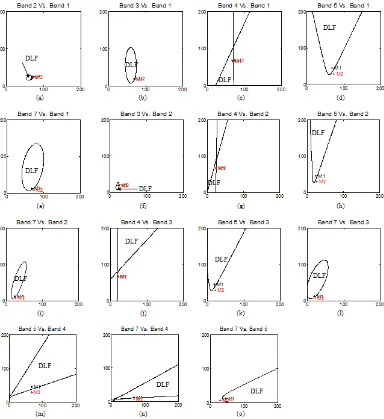
Fig. 5. Decision boundaries between coastal swamp forest and dryland forest for ML classification.
4 Conclusions
and mean brightness in all bands. The separation between mean of the classes in the decision space is believed to be one of the main factors that leads to the high classification accuracy of ML.
References
[1] A. Ahmad, and S. Quegan, Cloud masking for remotely sensed data
using spectral and principal components analysis, Engineering,
Technology & Applied Science Research (ETASR), 2 (2012), 221 – 225.
[2] ENVI, User’s guide, Research Systems Inc., USA, 2006.
[3] J. Scepan, Thematic validation of high-resolution global land-cover data sets, Photogrammetric Engineering and Remote Sensing, 65 (1999), 1051 – 1060.
[4] J.A. Richards, Remote sensing digital image analysis: An introduction. Springer-Verlag, Berlin, Germany, 1999.
[5] J.B. Campbell, Introduction to remote sensing, Taylor & Francis, London, 2002.
[6] J.R. Jensen, Introductory Digital Image Processing: A Remote Sensing
Perspective, Pearson Prentice Hall, New Jersey, USA, 1996.
[7] M. Story and R. Congalton, Accuracy assessment: a user's perspective,
Photogrammetric Engineering and Remote Sensing, 52 (1986), 397 –
399.
[8] S.A. Ackerman, K.I. Strabala, W.P. Menzel, R.A. Frey, C.C. Moeller and L.E. Gumley, Discriminating clear-sky from clouds with MODIS,
Journal of Geophysical Research, 103 (1998), 32141 – 32157.
[9] T.M. Lillesand, R.W. Kiefer and J.W. Chipman, Remote Sensing and
Image Interpretation, John Wiley & Sons, Hoboken, NJ, USA, 2004.