See discussions, stats, and author profiles for this publication at: https://www.researchgate.net/publication/220644280
Automatic eye fixations identification based on
analysis of variance and covariance
Article in Pattern Recognition Letters · October 2011
DOI: 10.1016/j.patrec.2011.06.012 · Source: DBLP
CITATIONS
6
READS
100
6 authors, including:
Giacomo Veneri
General Electric
18PUBLICATIONS 59CITATIONS SEE PROFILE
Pietro Piu
Università degli Studi di Siena
30PUBLICATIONS 92CITATIONS SEE PROFILE
Francesca Rosini
Università degli Studi di Siena
35PUBLICATIONS 127CITATIONS SEE PROFILE
Pamela Federighi
Università degli Studi di Siena
27PUBLICATIONS 92CITATIONS SEE PROFILE
Automatic Eye Fixations Identification based on
Analysis of Variance and Covariance
Giacomo Veneria,b,c,∗
, Pietro Piub
, Francesca Rosinib
, Pamela Federighia,b , Antonio Federicob, Alessandra Rufaa,b,∗
a
Eye tracking & Vision Applications Lab - University of Siena
b
Department of Neurological Neurosurgical and Behavioral Science - University of Siena
c
Etruria Innovazione Spa
Abstract
Eye movement is the simplest and repetitive movement that enables humans to interact with the environment. The common daily activities, such as reading a book or watching television, involve this natural activity, which consists of rapidly shifting our gaze from one region to another. In clinical application, the identification of the main components of eye movement dur-ing visual exploration, such as fixations and saccades, is the objective of the analysis of eye movements: however, in patients affected by motor control disorder the identification of fixation is not banal. This work presents a new fixation identification algorithm based on the analysis of variance and co-variance: the main idea was to use bivariate statistical analysis to compare variance over x and y to identify fixation. We describe the new algorithm, and we compare it with the common fixations algorithm based on dispersion. To demonstrate the performance of our approach, we tested the algorithm in a group of healthy subjects and patients affected by motor control disorder.
Keywords: Eye Tracking, Fixation identification, Analysis of Variance, Motor Control Disorder
∗Department of Neurological Neurosurgical and Behavioral Science - University of Siena, Viale Bracci 2, 53100 Siena, Phone +39-0577-233136, Fax +39-0577-40327
1. Introduction 1
Eye movements are an essential part of human vision as they drive the 2
fovea and, consequently, visual attention toward a region of interest in the 3
space. This enables visual system to process an image or its details with a 4
high resolution power (Privitera and Stark, 2000). 5
The study of eye movements is an up-and-coming tool to study neurolog-6
ical disorders in clinical applications. Voluntary eye movements (saccades, 7
smooth pursuit) are controlled by several structures in the central nervous 8
system, which may enable easier distinction between peripheral and central 9
lesions (Juhola et al., 2007). Brain’s structures of the paramedian pontine 10
reticular formation and the vestibulo-cerebellum are involved in the coor-11
dination of eye movements and in vestibular responses (Leigh R.J., 2006). 12
Some other neurological diseases, such as cerebellar ataxia, have an influence 13
on saccade velocity, accuracy or latency. 14
Therefore, a correct analysis of eye movements can lead to distinguish pa-15
tients from healthy subjects. 16
The fixations and saccades are the main features of eye movements; fixations 17
are samples of points around a centre point (centroid) with long duration 18
(>> 50ms); these eye fixations are intercalated by rapid eye jumps
(sac-19
cade), which can be defined as rapid eye movement with velocities that may 20
be higher than 500 deg/sec and duration about 20-40 ms (Ramat et al., 21
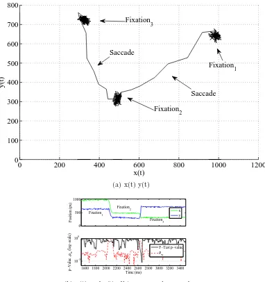
2007); Fig. 1 shows a small portion of gaze sample during visual exploration 22
on a psychological task: it’s easy to identify three clusters of data points 23
(fixations) and two saccades. 24
25
From a psychological point of view, the fixation is defined as the act 26
of maintaining the visual gaze on a single location in order to make our 27
environment visible (see Martinez-Conde et al. (2004) for a review of the role 28
of fixations). From a technical point of view, fixation should be identified by 29
a cluster of points around a centroid with a minimum duration; Irwin et al. 30
(1990) found the theoretical minimum duration for a single fixation to be 31
150 ms, whereas Manor and Gordon (2003) argued that 100 ms can also be 32
justified. Rayner (1998) indicated that the mean duration of a single fixation 33
may depend on the nature of the task (225 ms on reading, 275 ms on visual 34
search, 400 ms hand-eye coordination). 35
During fixation, the eye does not remain completely stable, but is affected by 36
0 200 400 600 800 1000 1200 0
100 200 300 400 500 600 700 800
x(t)
y(t)
Fixation 2 Saccade
Fixation 3
Fixation 1
Saccade
(a) x(t) y(t)
0 500 1000
Position (px)
1600 1800 2000 2200 2400 2600 2800 3000 3200 3400 10−5
100
p−Value ,
ρw
(log−scale)
Time (ms)
x y
F−Test p−value
ρw
Fixation
1
Fixation
2
Fixation
3
(b) x(t) and y(t), distance covariance and p-value (bottom graph).
Figure 1: A small portion of gaze of subject GV. For each sample (x(τ), y(τ)) at timeτ
making it difficult to easily identify it by an algorithm. 38
1.1. Related works 39
In order to implement an efficient algorithm able to identify automat-40
ically fixations, the efforts have been concentrated on three parameters : 41
fixations duration, dispersion and velocity. Generally speaking, the most 42
common algorithms are based on clustering analysis (Urruty et al., 2007) or 43
dispersion thresholding: Distance Dispersion Algorithm, Centroid-Distance 44
Method (Anliker, 1976), Position-Variance Method and Salvucci I-DT Algo-45
rithm (Salvucci and Goldberg, 2000). 46
In Distance Dispersion Algorithm each point in that fixation must be no 47
further than some threshold dmax from every other point. Position-Variance
48
requires that M of N points have a standard deviation of distance from the 49
centroid not exceeding σmax.Centroid-Distance requires that M of N points
50
be no further than some threshold from the centroid of the N points. Salvucci 51
I-DT requires that the maximal horizontal distance and the maximal vertical 52
distance is less than threshold. 53
Shic et al. (2008) accomplished a comparison of this algorithms: they found 54
that choices in analysis can lead to very different interpretations of the same 55
eye-tracking data. Blignaut (2009) found that the correct setting of disper-56
sion threshold on I-DT is of utmost importance, especially if the subjects are 57
not homogeneous. 58
1.2. Objective 59
We aimed to develop a robust algorithm able to identify fixations in clini-60
cal cases. The dispersion algorithm of I-DT Algorithm is accounted to be the 61
most robust method (Shic et al., 2008), we implemented the new algorithm 62
(Fixation Dispersion algorithm based on Covariance - C-DT) based on the 63
similar principle, but we evaluated the bivariate variance around the cen-64
troid and the covariance to classify the data point. In Veneri et al. (2010b) 65
we used the F-test of equal variance to identify fixations: the key principle 66
of the proposed technique was based on supposing the variance along the 67
x was not significantly different from that along the y during fixations: the 68
algorithm was able to identify more fixations than I-DT, but in clinical cases, 69
where eye movements should be affected by brain diseases, the assumptions 70
such as the normality of distribution or the number of data points should af-71
fect the efficacy of the algorithm. For these reasons we used a mixed method 72
The first section of the paper describes the implemented algorithm, then a 74
comparison between the C-DT and the I-DT Algorithm applied to simulated 75
(artificial) fixations is proposed; the final section is devoted to a case study 76
in normal subjects and patients. 77
2. Material and methods 78
2.1. Simulated fixations 79
In order to assess the proposed algorithm C-DT, we simulated 3500 fixa-80
tions plus a small portion of two saccades at the endpoint of fixation. Fixation 81
was defined as two dimensional sample vector data points x(t), y(t) around 82
the fixation’s centroidxc(t), yc(t), distributed with random Gaussian variance
83
Beers model (van Beers, 2008) with maximum velocity equal to 600 deg/s
85
(Ramat et al., 2007). 86
The duration of fixation ranged from 50 to 550ms. The variance over the x 87
and y ranged from 3 px2 to 50 px2, which corresponded to a max dispersion
88
ranging from 10pxto 300px. 89
2.2. Subjects’ fixations 90
Fourteen healthy subjects and six patients with (diagnosed and well 91
known) eye motor control disorder were enrolled aged 25-45. Subjects were 92
seated at viewing distance of 78cm from a 32” color monitor (51cm×31cm). 93
Eye position was recorded using ASL 6000 system, which consists of a remote-94
mounted camera sampling pupil location at 240Hz. A 9-point calibration and 95
3-point validation procedure was repeated several times to ensure all record-96
ings had a mean spatial error of less than 0.3degree. Data was controlled by 97
a Pentium4 dual core 3GHz computer, which acquires signals by fast UART 98
serial port. Head movement was restricted using a chin rest and bite. Sub-99
ject was asked to fixate a centered red dot on the center; after 500ms the 100
centered red dot disappeared and subject could explore the scene. The dis-101
played scenes were randomly choosen in a collection of real images (Privitera 102
and Stark, 2000) or pop-up images. The fixations were manually identified 103
by an expert operator. 104
3. Theory 106
In human visual search the source of variability should be due to the same 107
system (Beers, 2007; Veneri et al., 2011); the key principle of the proposed 108
technique is based on supposing x and y independent with the same variance 109
during a fixation. 110
The method is based on this assumption, and evaluates the hypothesis by 111
distance covariance coefficient and a statistical method such as the F-test 112
for equal variance; the F-test is used to verify that two populations (with 113
normal distribution) have the same mean or variance (this is the so called 114
”null hypothesis” H0 to be tested against the alternative complementary 115
hypothesis H1 that the two populations have heterogeneous variances) and 116
is a standard statistical procedure. In an informal way the F test calculates 117
the F distribution 118
between group variability
within group variability =
variability over x or y
variability between x y (1)
and, then, evaluates the probability to get a result of the test less than 119
the one actually observed when the null hypothesis H0 is true (in the C-DT 120
algorithm there is no difference between the two variances): this probability is 121
often indicated p-value or simply p. We must note that F-test was diagnosed 122
as being extremely sensitive to non-normality (Markowski, 1990). 123
We assumed that x and y on fixations come from a normal distribution with 124
same variance: then the highest relative p-values that did not accept the null 125
hypothesis (greater than 5%) were classified as the centroid of the fixation. 126
The assumption of equal variance and the normality of the distribution, may 127
be eligible for normal subjects, but in the case of patients affected by motor 128
control disorders, the fixation is affected by nystagmus, drifts, square jerks 129
(Leigh R.J., 2006) and the method should fail. Covariance is a measure of 130
how much the deviations of two or more variables or processes match and 131
should be a good candidate to replace or integrate the F-test. Covariance is 132
where x is the mean of vector x. If x and y are independent, then their 134
reasons the correlation coefficient (Sz´ekely et al., 2007) (or a bivariate non-136
parametric test (Feuerverger, 1993)) is more suitable. Correlation coefficient 137
is defined as 138
ρ(x, y) = cov(x, y)
σx·σy
(3)
whereσx and σy are the standard deviations of x and y respectively and
139
the product provides the normalisation factor to hold the Cauchy-Schwarz 140
inequality 0≤ρ(x, y)≤1. 141
Formally, the classification problem should be defined by: given a data point 142
x(t), y(t) at time t 1
143
x(t), y(t)→F if |ρ(x(τ), y(τ))| ≤k ∀τ ∈(t−w/2,t+w/2) (4)
where (t−w/2, t+w/2) is a small time window, Fis the set of fixations 144
andkis a constant (threshold)∈(0,1). From an intuitive point of view, when 145
x and y are randomly distributed, they are independent and ρ(x, y)≈0. 146
4. Calculation 147
The Eq. 4 is theoretically correct, but it was very sensitive to microsac-148
cade, small changes and depended strictly from k. We used a windowed 149
Pearson’s Correlation Coefficient defined as: 150
ρw(x, y,t) =
|cov(x(τ), y(τ))| σxσy
∀τ ∈(t−w/2,t+w/2) (5)
wherew was set to the minimum “physiological wave” to take in consid-151
eration, which is, in our case, the saccade: w= 20−25ms≈6sampleandσx
152
is the variance ofx. The Eq. 5 does not hold the Cauchy-Schwarz inequality, 153
but keeps the independent condition for ρw = 0.
154
To develop a more robust technique we integrated the proposed method with 155
an empirical mixed method based on covariance distance and F-test: 156
1
ξw(x, y,t) =
determining the degree of freedom and evaluating the F function = σ2 x/σ
2 y
159
with n-1 and n-1 degree of freedom and, finally, finding the p-value on the 160
F-distribution table. β is a very small empirical threshold ∼= 0.01, and α is 161
the standard confidence interval of p-value: α1 = 0.05 andα2 = 0.01. Finally
162
we applied Eq. 4 for 163
k =ξw(x, y,t) ∀(x(t), y(t)) when pw(x, y,t)> α1 (7)
From an intuitive point of view, k is evaluated as mean of Eq. 6 only for 164
consideration anything else than dispersion of fixations, avoiding any consid-170
eration on velocity or duration of fixation. 171
Starting from the centroid, the algorithm identifies the entire fixation 175
4.1. Algorithm description 179
In summary: (x,y) where F-test for equal variance accepts the H0 is in 180
are classified according to covariance and threshold k estimated through F-182
test for equal variance. The pseudo code A. 1 describes the algorithm: 183
1. the covariance distance and equal variance are evaluated on a small 184
time window (Eq. 6) 185
2. threshold constant k is estimated through F-test for equal variance 186
(Eq. 7) 187
3. the points (x,y) having the same variance or small covariance (≤k) are 188
assigned to fixations set (Eq. 4) 189
4. the fixations are group of contiguous points (Eq. 8) 190
5. the fixation is extended until variances product remains the same (Eq. 9) 191
5. Results 192
5.1. Simulated fixations 193
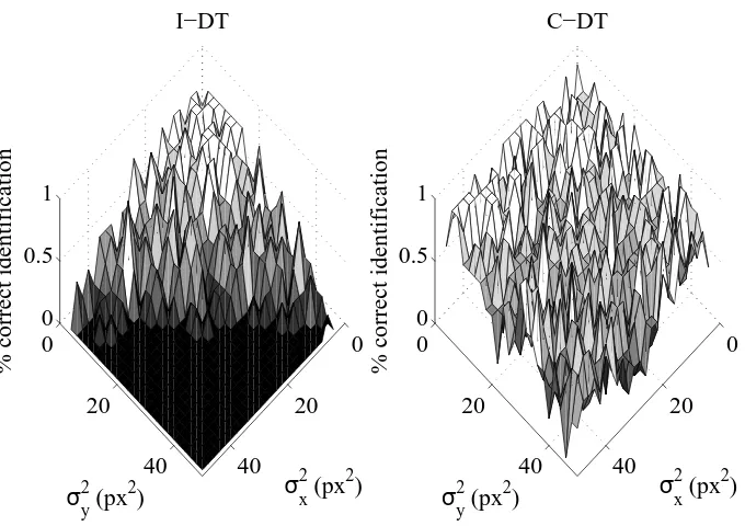
Fig. 2 and Fig. 3 show C-DT compared to I-DT. I-DT failed when dis-194
persion was greater than the maximum dispersion admitted by algorithm. 195
We cannot consider this being an error, but it’s the main characteristic of 196
the I-DT algorithm; similar result was found by Shic et al. (2008). The C-197
DT does not consider maximum dispersion, but only the covariance between 198
variance over x and y. 199
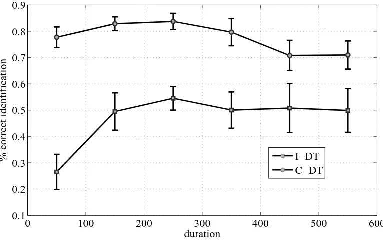
Generally speaking the C-DT identified simulated fixations with a preci-200
sion of 87% and I-DT of 42%. The performance of I-DT, however, strictly 201
depends on the threshold dispersion set; when we chose a large threshold 202
the I-DT identified more fixations, but in a real case should be affected by 203
incorrect clasification of saccade. 204
C-DT failed when it identified one fixation as two fixations (over segmenta-205
tion problem). 206
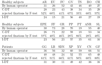
5.2. Case study 207
The fixations of fourteen healthy subjects and six patients with cerebellar 208
disorders were analyzed: C-DT identified 88,11% of fixations. I-DT was set 209
to max dispersion threshold (∼= 110px) and identified 63,86% of fixations. 210
The algorithms I-DT and C-DT were applied to raw data; when we applied 211
a low-pass filter (Butter-worth filter, 3rd order, fc = 2.1Hz) the
perfor-212
mances improved to∼93%, but it depends from the type of filter and filter’s 213
0
20
40 0
20
40 0
0.5 1
σx2 (px2) I−DT
σy2 (px2)
% correct identification
0
20
40 0
20
40 0
0.5 1
σx2 (px2) C−DT
σy2 (px2)
% correct identification
Figure 2: Percentage of correctly identified fixations by I-DT and C-DT varying variance of x axis, y axis and duration of fixation. Performance of I-DT and C-DT are similar for small values of σx and σy; when dispersion of x and/or y increased (max dispersion varied 150pxto 300px) I-DT was not able to identify fixation as expected, on the contrary, performance of C-DT remained stable. Performance of C-DT appeared to decrease when
0 100 200 300 400 500 600 0.1
0.2 0.3 0.4 0.5 0.6 0.7 0.8 0.9
% correct identification
duration
I−DT C−DT
Healthy subjects AR EU FC GV TS BO CH
By human operator 31 26 52 43 46 40 27
C-DT 28 23 43 38 34 35 29
rejected fixations by F-test 52% 60% 41% 67% 35% 60% 57%
I-DT 24 15 21 56 40 27 19
Healthy subjects EPE FF GR PP PT ANR SL
By human operator 30 73 28 70 19 55 40
C-DT 26 71 22 59 18 53 34
rejected fixations by F-test 57% 40% 46% 28% 86% 28% 48%
I-DT 23 56 23 57 35 61 16
Patients GG LB SDN XP XV CN GF
By human operator 36 56 32 60 59 66 51
C-DT 40 48 24 52 55 65 48
rejected fixations by F-test 61% 51% 66% 61% 50% 60% 80%
I-DT 31 30 11 49 42 36 16
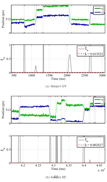
Figure 4 shows a small portion of gaze of subject GV and EU. C-DT 215
identified ∼= 90% of fixations. 216
217
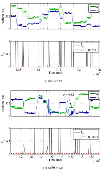
Figure 5 shows a small portion of an exploration made by subject FC and 218
AR: C-DT identified the fixations (thick line) also on high variance cases. 219
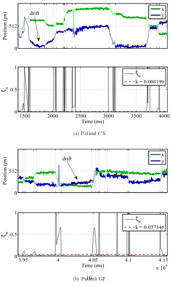
Figure 6 shows the exploration made by patients: C-DT was insensitive 220
to drifts, but failed for artifacts such as spikes. 221
An empirical analysis of lost fixations was performed; I-DT failed to iden-222
tify correctly large fixations or very short fixations (≤60ms). The short fixa-223
tions, however, are classified by some authors saccade interruptions (Findlay 224
et al., 2001). C-DT failed on the identification a single fixation as two or more 225
fixations (over segmentation problem) or on grouping two fixations separated 226
by a very small saccade. In any case, a close comparison between I-DT and 227
C-DT does not make sense because they work with different techniques and 228
very often it is not trivial to define a “fixation”. 229
6. Conclusion 230
In the last decade a large effort has been made to identify fixations (An-231
liker, 1976; Salvucci and Goldberg, 2000; Urruty et al., 2007; Blignaut, 2009), 232
however it is not yet easy to provide a formal mathematical definition of fix-233
ation: some authors have demonstrated that fixation’s parameters depend 234
strictly by the type of task (Rayner, 1998; Irwin et al., 1990; Manor and Gor-235
don, 2003; Shic et al., 2008). We suggested a formal definition of fixations 236
based on analysis of variance between x axis and y axis; the implemented 237
algorithm is based on the dispersion algorithm I-DT developed by Salvucci 238
and Goldberg (2000) and integrates it with a statistical test (F-test) and 239
covariance. The main advantage of the proposed technique is to provide a 240
new definition of fixation which does not require the setting of any critical 241
parameter or threshold, and provides a probability value of correctness. 242
Further work will be addressed to improve the extension mechanism described 243
in the algorithm 1 by a robust method such as the correntropy. Then, to avoid 244
the normality assumption, the F-test should be replaced by a non paramet-245
ric test, but it will require more points. Then, due to the high sensitivity of 246
F-test, we will evaluate the opportunity to integrate it on a real-time appli-247
cation such as gaze-contingent (Veneri et al., 2010a). 248
Finally we will investigate towards improving the system of recognition of 249
0 512
Position (px)
x y
500 1000 1500 2000 2500 3000
0 0.5 1
Time (ms) ξ w
ξw
k = 0.015822
(a) Subject GV
0 512
Position (px)
x y
4.2 4.25 4.3 4.35 4.4 4.45
x 104 0
0.5 1
Time (ms) ξ w
ξw
k = 0.002827
0 512
Position (px)
x y
4.05 4.1 4.15 4.2 4.25
x 104 0
0.5 1
Time (ms) ξ w
ξw
k = 0.002511
(a) Subject FC
0 512
Position (px)
x y
4.2 4.25 4.3 4.35 4.4 4.45 4.5 4.55 x 10⁴ 0
0.5 1
Time (ms) ξ w
ξ
w
k = 0.025633
σ = 6.82
0 512
Position (px)
x y
1500 2000 2500 3000 3500 4000
0 0.5 1
Time (ms) ξ w
ξw
k = 0.008190 drift
(a) Patient CN
0 512
Position (px)
x y
3.95 4 4.05 4.1 4.15
x 104 0
0.5 1
Time (ms) ξ w
ξ
w
k = 0.037346 drift
patients with severe ocular motor disorders such as nystagmus or tremor 251
(Federighi et al., 2011). In this kind of patients the source of variability 252
of fixations should be different between x and y and the algorithm should 253
fail; the difference, however, depends strictly on the subject and the ratio of 254
variability between x and y should be calculated a priori. 255
Acknowledgment 256
The authors would like to thank the editor and reviewers for improvements
257
and suggestions and Tuscany Region and Grado Zero Espace (Dr. Matteo Piccini)
258
for funding support (SISSI Project) on the current research.
259
Materials 260
Developed MATLAB algorithm should be downloaded at [THE JOURNAL
261
URL].
262
Appendix A. Algorithm 263
References 264
Anliker, L., 1976. Eye movements: On-line measurement, analysis, and control.
265
Eye movements and psychological processes , 185–199.
266
Beers, R.J., 2007. The sources of variability in saccadic eye movements. Journal
267
of Neuroscience 27, 8757–8770.
268
van Beers, R.J., 2008. Saccadic eye movements minimize the consequences of
269
motor noise. PLoS One 3, e2070.
270
Blignaut, P., 2009. Fixation identification: the optimum threshold for a dispersion
271
algorithm. Atten Percept Psychophys 71, 881–895.
272
Federighi, P., Cevenini, G., Dotti, M.T., Rosini, F., Pretegiani, E., Federico, A.,
273
Rufa, A., 2011. Differences in saccade dynamics between spinocerebellar ataxia
274
2 and late-onset cerebellar ataxias. Brain 134, 879–891.
275
Feuerverger, A., 1993. A consistent test for bivariate dependence. International
276
Statistical Review / Revue Internationale de Statistique 61, pp. 419–433.
Algorithm 1 Operator ”a:b” means ”all point between a and b”. Operator ”cov”, ”var” or ”ftest” are the functions which evaluates covariance, variance of a vector and ftest of two vectors. Operator ”relativemax” is a function which calculates the relative maximum of contiguous points.
1: {Calculate variance} 2: σx←var(x)
3: σy←var(y)
4: for all x(t), y(t) do
5: xˇ←x(t−w/2) :x(t+w/2) 6: yˇ←y(t−w/2) :y(t+w/2)
7: F(t)←f test(ˇx,yˇ){F-test on datax(t), y(t)t∈(−w/2, w/2)}
8: R(t)← |cov(ˇx,yˇ)|/(σxσy) 9: t←t+ ∆t{Move to next point} 10: if F(t)≥0.05 ANDR(t)≤0.01then
11: R(t)←0
12: end if
13: if F(t)≤0.01 ANDR(t)≥0.01then
14: R(t)←1
15: end if
16: end for
17: {Evaluate threshold}
18: χ←mean(R(τ))∀τ:F(τ)≥0.05 19: {Identify fixations centroid} 20: R∗←R≤χ
21: {Look for centroids}
22: xi, yi←relativemax(x(t), y(t), R∗)
23: {Extend fixation}
24: for all xi, yi do
25: xˇ←x(t−w/2) :x(t+w/2) 26: yˇ←y(t−w/2) :y(t+w/2)
27: {Calculate product of variances of x and y on data (xt, yt)t∈(−W, W)} 28: s←var(ˇx)·var(ˇy)
29: ss←s
30: t0←t−w/2
31: t1←t+w/2
32: while ss≤sAND CONTINUEdo
33: xx←x(t0−∆t) :x(t1)
34: yy←y(t0−∆t) :y(t1)
35: ss←var(xx)·var(yy) 36: if ss≤sthen
37: t0←t0−∆t
38: CONTINUE
39: end if
40: xx←x(t0) :x(t1+ ∆t)
41: yy←y(t0) :y(t1+ ∆t)
42: ss←var(xx)·var(yy) 43: if ss≤sthen
44: t1←t1+ ∆t
45: CONTINUE
46: end if
47: end while
Findlay, J.M., Brown, V., Gilchrist, I.D., 2001. Saccade target selection in visual
278
search: the effect of information from the previous fixation. Vision Res 41,
279
87–95.
280
Hogg, R.V., Ledolter, J., 1987. Engineering Statistics. MacMillan.
281
Irwin, D.E., Zacks, J.L., Brown, J.S., 1990. Visual memory and the perception of
282
a stable visual environment. Percept Psychophys 47, 35–46.
283
Juhola, M., Aalto, H., Hirvonen, T., 2007. Using results of eye movement signal
284
analysis in the neural network recognition of otoneurological patients. Comput.
285
Methods Prog. Biomed. 86, 216–226.
286
Leigh R.J., Z.D., 2006. The neurology of eye movements (Book/DVD). Fourth
287
edition. New York: Oxford University Press.
288
Manor, B.R., Gordon, E., 2003. Defining the temporal threshold for ocular fixation
289
in free-viewing visuocognitive tasks. J Neurosci Methods 128, 85–93.
290
Markowski, Carol A; Markowski, E.P., 1990. Conditions for the effectiveness of a
291
preliminary test of variance. The American Statistician 44, 322326.
292
Martinez-Conde, S., Macknik, S.L., Hubel, D.H., 2004. The role of fixational eye
293
movements in visual perception. Nature Reviews Neuroscience 5, 229–240.
294
Privitera, C., Stark, L., 2000. Algorithms for defining visual regions-of-interest:
295
comparison with eye fixations. Pattern Analysis and Machine Intelligence, IEEE
296
Transactions on 22, 970–982.
297
Ramat, S., Leigh, R.J., Zee, D.S., Optican, L.M., 2007. What clinical disorders
298
tell us about the neural control of saccadic eye movements. Brain 130, 10–35.
299
Rayner, K., 1998. Eye movements in reading and information processing: 20 years
300
of research. Psychol Bull 124, 372–422.
301
Salvucci, D.D., Goldberg, J.H., 2000. Identifying fixations and saccades in
eye-302
tracking protocols, in: ETRA ’00: Proceedings of the 2000 symposium on Eye
303
tracking research & applications, ACM, New York, NY, USA. pp. 71–78.
304
Shic, F., Scassellati, B., Chawarska, K., 2008. The incomplete fixation measure,
305
in: ETRA ’08: Proceedings of the 2008 symposium on Eye tracking research
306
and applications, ACM, New York, NY, USA. pp. 111–114.
Sz´ekely, G.J., Bakirov, N.K., Rizzo, L.M., 2007. Measuring and testing
indepen-308
dence by correlation of distances. The Annals of Statistics 35, 2769–2794.
309
Urruty, T., Lew, S., Djeraba, C., Simovici, D.A., 2007. Detecting eye fixations by
310
projection clustering, in: Proc. 14th International Conference on Image Analysis
311
and Processing Workshops ICIAPW 2007, pp. 45–50.
312
Veneri, G., Federighi, P., Rosini, F., Federico, A., Rufa, A., 2010a. Influences of
313
data filtering on human-computer interaction by gaze-contingent display and
314
eye-tracking applications. Computers in Human Behavior 26, 1555 – 1563.
315
Veneri, G., Federighi, P., Rosini, F., Federico, A., Rufa, A., 2011. Spike removal
316
through multiscale wavelet and entropy analysis of ocular motor noise: A case
317
study in patients with cerebellar disease. Journal of Neuroscience Methods 196,
318
318–326.
319
Veneri, G., Piu, P., Federighi, P., Rosini, F., Federico, A., Rufa, A., 2010b. Eye
320
fixations identification based on statistical analysis - case study, in: Cognitive
321
Information Processing (CIP), 2010 2nd International Workshop on, IEEE. pp.
322
446 –451.