IDENTIFICATION SEAGRASS CONDITION FROM ALOS
AVNIR-2 USING ARTIFICIAL NEURAL NETWORK
AT PARI ISLAND
AMRAN FIRDAUS
GRADUATE SCHOOL
BOGOR AGRICULTURAL UNIVERSITY
BOGOR
STATEMENT
I, Amran Firdaus, hereby declare that this thesis entitled
Identification Seagrass Condition from ALOS AVNIR-2
Using Artificial Neural Network at Pari Island
Is a result of my own work under the supervision advisory board and that it has
not been published before. The content of the thesis has been examined by the
advising the advisory board and external examiner
Bogor, May 2011
Amran Firdaus
ABSTRACT
AMRAN FIRDAUS. Identification Seagrass Condition from ALOS AVNIR-2 using Artificial Neural Network at Pari Island. Under the supervision of KUDANG B SEMINAR and ANTONIUS B WIJANARTO.
Seagrass beds have important roles in marine life, but the unavailable of information about the condition of seagrass causes difficulties in managing coastal areas properly. Regularly updated and accurate information on the percentage cover of seagrass is an essential component of the knowledge required to monitor, understand and manage this resource. Artificial Neural Network (ANN) was applied to ALOS AVNIR-2 to identify seagrass condition. Twenty two classification scenarios were done to compare the result of accuracy. There are three class of seagrass condition. Seagrass cover more than 60% indicates the condition of good seagrass. Seagrass cover from 30% to 59,9% indicates the condition of medium seagrass. Seagrass cover below 29,9% indicates the condition of poor seagrass.
Best accuracy was obtained by scenario H by entering combination of blue (0.42 to 0.50 μm) and NIR (0.76 to 0.89 μm) wavelength plus water depth data as input parameters, with a value of 71.43% overall accuracy. However, looking at individual class, Scenario C, which is 58.33% of overall accuracy by using combination of blue (0.42 to 0.50 μm), green (0.52 to 0.60 μm), NIR (0.76 to 0.89 μm) wavelength plus water depth achieved higher producer and user accuracy. Overall, the result of identification seagrass condition from ALOS AVNIR-2 using artificial neural network at Pari Island in 2010 is dominated by poor seagrass, while good seagrass and medium seagrass were found in small area.
ABSTRAK
AMRAN FIRDAUS. Identification Seagrass Condition from ALOS AVNIR-2 using Artificial Neural Network at Pari Island. Dibimbing oleh KUDANG B SEMINAR dan ANTONIUS B WIJANARTO.
Padang lamun memiliki peran penting dalam kehidupan laut, namun tidak tersedianya informasi tentang kondisi padang lamun menyebabkan kesulitan dalam mengelola kawasan pesisir dengan benar. Memperperbaharui secara teratur dan akurat tentang informasi luas tutupan lamun merupakan hal yang penting dari pengetahuan yang dibutuhkan untuk memantau, memahami dan mengelola sumberdaya ini. Artificial Neural Network (ANN) telah diterapkan pada ALOS-AVNIR 2 untuk mengetahui kondisi lamun. Dua puluh dua skenario klasifikasi dilakukan untuk membandingkan hasil akurasi. Ada tiga kelas kondisi lamun. Tutupan lamun lebih dari 60% menunjukkan kondisi padang lamun baik. Tutupan lamun dari 30% sampai 59,9% menunjukkan kondisi lamun sedang. Tutupan lamun dibawah 29,9% menunjukkan kondisi lamun jelek.
Hasil akurasi terbaik diperoleh oleh skenario H yang memasukan kombinasi panjang gelombang biru (0.42 to 0.50 μm), dan NIR (0.76 to 0.89 μm) ditambah data kedalaman air sebagai parameter masukan, dengan nilai keseluruhan akurasi 71,43%. Namun, melihat kelas individu, Skenario C, dengan nilai akurasi keseluruhan 58,33% yang menggunakan kombinasi panjang gelombang biru (0.42 to 0.50 μm), hijau (0.52 to 0.60 μm), NIR (0.76 to 0.89 μm) ditambah data kedalaman air mencapai nilai lebih tinggi untuk akurasi produser dan pengguna. Secara keseluruhan, hasil identifikasi kondisi lamun dari ALOS AVNIR-2 menggunakan artificial neural network di Pulau Pari tahun 2010 didominasi oleh lamun jelek, sedangkan lamun baik dan sedang ditemukan di sebagian kecil area.
SUMMARY
AMRAN FIRDAUS. Identification Seagrass Condition from ALOS AVNIR-2 using Artificial Neural Network at Pari Island. Under the supervision of KUDANG B SEMINAR and ANTONIUS B WIJANARTO.
Seagrass ecosystems are important and critical habitat for the survival of marine biota of life, even to advocate one alternative livelihood and income of the community who have long lived in coastal areas. Seagrass meadows produce a variety of goods (finfish and shellfish) and provide ecological services (maintenance of marine biodiversity, regulation of the quality of coastal waters, protection of the coast line) which are directly used or beneficial to humans and condition the economic development of Indonesian coastal zones. On the other hand, seagrass is also sensitive to various human activities such as reclamation, adding the port, making jeti, settlements, surface flow, the waste industry and coastline unstable. Understanding the extent and condition of these seagrass meadows and how they change over time is essential for their management and sustainable use.
Considering to the very extensive area to be studied, for obtaining precise information of Indonesian seagrass coverage, it is favorable to use remote sensing technique as alternative tool. In Indonesia, particularly seagrass identification using satellite imagery is still rarely done. The objective of this research is to identify the seagrass condition from ALOS AVNIR-2 using Artificial Neural Network classification scenario.
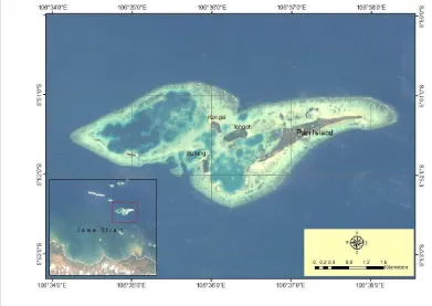
Study area in this research is located in Jakarta Province, Seribu Island District, precisely in Pari Island covering Burung Island, Tengah Island, and Kongsi Island. Pari Island has depth range between 0-50 meters, which the physics and chemical parameter of water has a good range where the seagrass can live. Seagrass meadow on Pari Island is the vegetation that lives in shallow waters. Pari Island is also having an important livelihood for almost the entire community surrounding it, which depends on seaweed farming and fishing.
Seagrass cover is a parameter to determined seagrass condition based on declaration of environment minister number 200/2004. There are three classifications of seagrass condition; 1) seagrass more than 60% indicates the condition of good seagrass, 2) seagrass cover from 30% to 59,9% indicates the condition of medium seagrass, and 3) seagrass cover below 29,9% indicates the condition of poor seagrass. Seagrass cover is referred to as the horizontally projected foliage cover of the seagrass canopy, which is recognized as a key information requirement for seagrass monitoring.
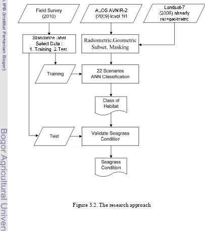
There are three main steps to identifying seagrass condition: image pre-processing, image classification, and accuracy assessment. In this study, geometric correction and atmospheric correction was applied before image classification, including subset and masking image. On image classification stage, some data observation and measurement from field survey directly will be used for ANN classification, and another will used for validation. Forty eight points of field data were divided into two data sets: 26 in the training data set and 22 in the testing. In this research, ANN supervised classification was guided by variety of input data sets including field survey, satellite imagery and expert knowledge to produce seagrass condition map. Twenty two scenario processes were done to compare the result of accuracy.
Field data were used to determine training sites for three levels of seagrass cover classes ( ≤ 29,9%, 30-59,9%, ≥ 60% ) in the ANN supervised image classification process. Reflectance signatures for each of the three different seagrass cover classes were extracted from the ALOS AVNIR-2 scene of Pari Island for the calibration field sites, which served as training sites for the image classification process. Characteristic spectral reflectance signatures were defined for each of the target levels of seagrass cover to be mapped.
Classification scenarios were developed to identify the seagrass condition at Pari Island. For this purpose, shallow water habitat was classified into nine classes; sea, sand, lagoon, coral, reef slope, mix habitat (coral, seagrass, seaweed, and sand), poor seagrass, medium seagrass, and good seagrass. The separability of ROIs between good seagrass and other habitat (poor seagrass, lagoon, sea, sand, coral, mix habitat, and reef slope) are 2.0, except between good seagrass and medium seagrass is 1.99. The separability between medium seagrass and other habitat (poor seagrass, lagoon, sea, sand, coral, mix habitat, and reef slope) are 1.93, 2.0, 2.0, 1.68, 1.88, 1.96 and 2.0 respectively. Value 2.00, 2.00, 2.00, 1.97, 1.95, and 2.00 are achieved between poor seagrass and lagoon, sea, sand, coral, mix habitat, and reef slope respectively. From that value of separability, two lower separability values got between medium seagrass and sand (1.68), and medium seagrass and coral (1.88).
From all of the classification scenarios that have been conducted, the results obtained accuracy varies for each scenario. Half of the accuracy of classification scenarios has value zero, while others were worth an average accuracy of 50%. The best accuracy was achieved by using combination of blue (0.42 to 0.50 μm) and NIR (0.76 to 0.89 μm) wavelength plus water depth, with an overall accuracy of 71.43%. However, looking at individual class, the classification scenario that used blue (0.42 to 0.50 μm), green (0.52 to 0.60 μm), NIR (0.76 to 0.89 μm) wavelength plus water depth achieved higher producer and user accuracy. Even NIR wavelengths are absorbed by water, but in this study this wavelength (0.76 to 0.89 μm) can be used for the habitat classification. It can be caused the water depth which was below 2 meters.
Furthermore, to improve the identification seagrass condition, it is important to explore the ability of ANN classification method itself, by changing the settings of the neural network training (training momentum, training rate, etc.). It would be better to use some of the satellite imagery with dissimilar sensor and different spatial resolutions to make a compare fine analysis of the results of classification. This is expected to obtain higher accuracy.
Copyright © 2011, Bogor Agricultural University Copyright are protected by law,
1. It is prohibited to cite all of part of this thesis without referring to and mentioning the source;
a. Citation only permitted for the sake of education, research, scientific writing, report writing, critical writing or reviewing scientific problem.
b. Citation does not inflict the name and honor of Bogor Agricultural University.
IDENTIFICATION SEAGRASS CONDITION FROM ALOS
AVNIR-2 USING ARTIFICIAL NEURAL NETWORK
AT PARI ISLAND
AMRAN FIRDAUS
A thesis submitted for the degree Master of Science in Information Technology
for Natural Resources Management Program Study
GRADUATE SCHOOL
BOGOR AGRICULTURAL UNIVERSITY
BOGOR
Research Title : Identification Seagrass Condition from ALOS AVNIR-2
using Artificial Neural Network at Pari Island
Name : Amran Firdaus
Student ID : G051080051
Study Program : Master of Science in Information Technology for Natural
Resources Management
Approved by,
Advisory Board
Prof. Ir. Kudang B. Seminar, M.Sc., Ph.D. Dr. Antonius B. Wijanarto
Supervisor Co-Supervisor
Endorsed by,
Program Coordinator Dean of Graduate School
Dr. Ir. Hartrisari Hardjomidjojo, DEA Dr. Ir. Dahrul Syah, M.Agr.Sc
Date of Examination: Date of Graduation:
ACKNOWLEDGMENTS
Alhamdulillah, first of all, the writer would like to express his grateful to Allah Subhanahu Wata’ala, Rab, God – Almighty for His blessing and mercy which has been given to the writer so that this research of thesis could be accomplished well. The success of this study would not have been possible without various contribution and support from many people and I will not be able to mention them one by one. Of course, I would like to express my highly appreciation to all of them.
I wish to thank my supervisor Prof Dr Kudang B Seminar, and my co-supervisor, Dr Antonius B Wijanarto for their guidance, technical comment and constructive critics through all months of my research.
Special words of thanks are due to Dr. Ibnu Sofian for providing important data and Dr Vincentus Siregar for valuable suggestion during the last stage of the work.
I would like also thank to all my colleagues in MIT and RCO LIPI for helping, supporting, and togetherness in finishing our study.
CURRICULUM VITAE
The Author was born in Bandung, West Java, Indonesia on July
21st 1972 He finished his bachelor degree from Indonesian
Institute of Technology on 2001. He has accepted as staff
Research Centre for Oceanography on 2001. He was entered the
IPB Graduate School in year 2008. He was enrolled as private
student in Master of Sciences in Information Technology for Natural Resources
Management, Bogor Agricultural University in 2008 and completed his master
study in 2011. His final thesis is “Identification Seagrass Condition from ALOS
i
TABLE OF CONTENT
TABLE OF CONTENT ... i
LIST OF TABLE ... iii
LIST OF FIGURE ... iv
LIST OF APPENDICES ... v
I. INTRODUCTION ... 1
1.1. Background ... 1
1.2. Objectives ... 3
1.3. Scope of Study ... 3
1.4. Problem Statement ... 4
1.5. Research Output ... 4
II. LITERATURE REVIEW ... 5
2.1. Seagrass ... 5
2.2. Remote Sensing... 7
2.3. Advance Land Observing Satellite (ALOS) ... 8
2.3.1. Advance Visible and Near Infrared Radiometric Type 2 ... 8
2.4. Remote Sensing Application for Seagrass Identification ... 10
2.5. Artificial Neural Network ... 11
2.6. Accuracy Assessment ... 14
III. METHODOLOGY... 17
3.1. Time and Location ... 17
3.2. Material and Tools ... 18
3.2.1. Data Source ... 18
3.2.2. Required Tools ... 18
3.3. Research Step ... 18
3.3.1. Image Preprocessing ... 20
3.3.2. Image Classification ... 20
ii
IV. RESULT AND DISCUSSIONS ... 25
4.1. General Condition ... 25
4.2. Image Preprocessing ... 26
4.2.1. Field Survey ... 28
4.2.2. Region of Interest (ROIs) ... 29
4.3. Image Classification ... 30
4.4. Accuracy Assessment ... 32
V. CONCLUSION AND RECOMMENDATIONS ... 37
5.1. Conclusion ... 37
5.2. Recommendation ... 38
iii
LIST OF TABLE
Table 2.1 Classification of Seagrass ... 6
Table 2.2 AVNIR-2 Characteristics ... 9
Table 2.3 Product Processing Definition ... 9
Table 2.4 Example of an Error Matrix ... 16
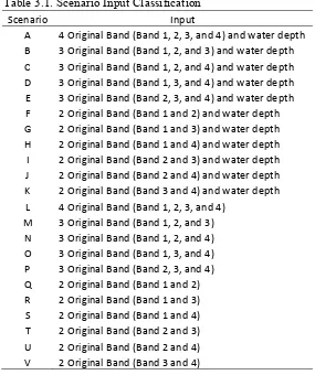
Table 3.1. Scenario Input Classification ... 21
Table 3.2. Neural Network Parameter ... 23
Table 4.1 Statistic before and after radiometric correction ... 27
Table 4.2 Accuracy Assessment ... 32
Table 4.4 Matrix of overall accuracy (Scenario H) ... 33
Table 4.5 Producer and User Accuracy (Scenario H) ... 34
Table 4.6 Producer and User Accuracy (Scenario C) ... 34
Table 4.7 Producer and User Accuracy (Scenario D) ... 34
iv
LIST OF FIGURE
Figure 2.1. The pathways of light over and in a shallow water system. ... 7
Figure 3.1. Study Area ... 17
Figure 3.2. The research approach ... 19
Figure 3.3. Structure of Backpropagation Neural Network ... 22
Figure 4.2 Subset of remote sensed data to focus at region of interest. ... 28
Figure 4.4. Plot of Neural Network Classification ... 31
Figure 4.5 ANN Habitat Classifications in Pari Island in 2010 (Scenario A) ... 31
v
LIST OF APPENDICES
1 I. INTRODUCTION
1.1.Background
The large knowledge about the biology and ecology of seagrass gained
during the last third of the 20th century has driven increased awareness of the
economic value of seagrass to humans. Seagrass feature high rates of primary
production. As any other photosynthetic organism, seagrass fix carbon dioxide
using the energy provided by light and transform it into organic carbon to sustain
seagrass growth and biomass production. High rates of biomass production imply
high rates of oxygen production, a byproduct of photosynthesis, which is released
to the surrounding waters.
Seagrass ecosystems are important and critical habitat for the survival of
marine biota of life, even to advocate one alternative livelihood and income of the
community who have long lived in coastal areas. In addition seagrass meadows
also have several functions, among which is a trap for sediment, reducing abrasion
coast, fisheries production support, as the habitat of various types of biota (flora
and fauna) sea coast. On the other hand, seagrass is also sensitive to various
human activities such as reclamation, adding the port, making jeti, settlements,
surface flow, the waste industry and coastline unstable (Short and Echeverria
1996, Duarte 2002).
In several areas of Indonesia, seagrass coverage and its distribution has been
change from time to time. For having so many islands and long coastal areas, it
was roughly estimated that approximately 30,000 km2 of seagrass cover
Indonesian Archipelago (Kuriandewa et al., 2003). However, reliable data of such information is inadequately available, since former and recent seagrass researches
rarely measured the extent of seagrass intentionally; they mainly focused on the
biology of seagrass and its associated biota (Hutomo, Kiswara and Azkab 1988).
Pari Island has depth range between 0-50 meters, which the physics and
chemical parameter of water has a good range where the seagrass can live. Pari
Island stand on coral reef flat with others islands on it, namely the Burung Island,
2
lagoon, and three complete tropical ecosystems such as mangroves, seagrass beds,
and coral, including the diversity of biological resources (fish, crustaceans,
mollusca, echinoderms, and seaweed) were quite abundant until the early 1980's
(Wouthuyzen et al.,2008). Therefore, Pari Island was set as an observation station marine science (particularly coastal areas) since 1970. In addition, Pari Island is
also having an important livelihood for almost the entire community surrounding
it, which depends on seaweed farming and fishing. The study conducted in
2008 by Wouthuyzen about the overall status evaluating ecosystems and living
resources in Pari Island showed that the biological resources in the cluster Pari
Island experienced a drastic decrease in symptoms. If it occurs continuously,
it can be expected to further decline of biological resources at Pari Island, which
impact on decreasing the catch of fishermen and people's income Pari Island.
Remote sensing for identification of seagrass has many advantages when
compared to conventional survey methods, which may include spatial only a
narrow area. Mapping of seagrass properties from remote sensing and/or field data
has been conducted in other tropical, sub-tropical and temperate environments.
ALOS AVNIR-2 is a visible and near-infrared radiometer for observing land and
coastal zones and provides better spatial resolution. It will be useful for
monitoring the condition of coastal resources such as mangrove forests, seagrass
meadows, coral reefs, coastal line change, and water quality. Seagrass extent was
mostly measured using rough estimation technique. Considering to the very
extensive area to be studied, for obtaining precise information of Indonesian
seagrass coverage, it is favorable to use remote sensing technique as alternative
tool.
Research on mapping and monitoring of shallow-water ecosystems have
been carried out using satellite image data (McKenzie et al. 2001). But in Indonesia, particularly the seagrass identification using satellite imagery is still
rarely done, only a few locations that have been done, including the east coast
Bintan Island in Riau Islands, Lembeh Strait and North Minahasa in North
Sulawesi, Sanur Beach in Bali, Gili Lawang and Gili Sulat in Lombok Island, and
3 Over the years, a number of classifications have been applied to produce
maps of the seagrass beds for a range of scientific and management purposes. The
most commonly used classification methods in remote sensing are statistical
classification algorithms such as the minimum distance and the maximum
likelihood. Although widely used, conventional statistical classification
techniques may not always be appropriate for mapping from remotely data. These
2 methods have their restrictions, related particularly to distributional assumptions
and to limitations on the input data types (Foody 1999).
The Artificial Neural Network (ANN) has seen a lot of interest from past few
years. It has been successfully applied to a wide range of domains such as finance,
medicine, engineering, geology and physics. Kaul et al, (2005), stated that many authors reported better accuracy when classifying spectral images with an ANN
approach than with a statistical method such as maximum likelihood. Neural
networks, with their ability to learn by example make them very flexible and
powerful. However, a more important contribution of the ANNs is their ability to
incorporate additional data in the classification process. A limited amount of
research has been conducted on the application of neural networks to identify
seagrass condition. Respond to this matter and to provide descriptive information
for proposed management of seagrass ecosystem, identification of seagrass
condition was carried out in Pari Island using remote sensing technique and ANN
classification.
1.2.Objectives
The objective of this research is to identify the seagrass condition from
ALOS AVNIR-2 using Artificial Neural Network classification scenario.
1.3.Scope of Study
1. Location: Pari Island is located at the position 1060 34’ 0” – 1060 38’ 0”
East Longitude and 050 52’ 50” – 050 54’ 50” South Latitude, Jakarta
province.
2. Data analysis in this study focus only seagrass condition based on
4
1.4.Problem Statement
The reason why choose seagrass is due to an important role in marine life,
but the unavailable of information about the condition of seagrass causes
difficulties in managing coastal areas properly. Seagrass meadows produce a
variety of goods (finfish and shellfish) and provide ecological services
(maintenance of marine biodiversity, regulation of the quality of coastal waters,
protection of the coast line) which are directly used or beneficial to humans and
condition the economic development of Indonesian coastal zones. Understanding
the extent and condition of these seagrass meadows and how they change over
time is essential for their management and sustained use. Regularly updated and
accurate information on the percentage cover of seagrass is an essential
component of the knowledge required to monitor, understand and manage this
resource.
1.5.Research Output
The output of this research is information about the condition of seagrass in
Pari Island – Seribu Island, which can be used as a reference for managing coastal
5
II. LITERATURE REVIEW
2.1.Seagrass
Seagrass are marine flowering plants (angiosperms); thus they live and
complete their entire life cycle submerged in seawater (including underwater
flowering, pollination, distribution of seeds and germination into new plants).
Seagrass also propagate vegetative by elongating their rhizomes; a whole meadow
may be one single clone resulting from one seedling. Both sexual reproduction
and vegetative growth are critical to the propagation and maintenance of seagrass
meadows (Hemminga and Duarte 2000).
Seagrasses have had many traditional uses (Terrados and Borum, 2004).
They have been used for filling mattresses (with the thought that they attract fewer
lice and mites than hay or other terrestrial mattress fillings), roof covering, house
insulation and garden fertilizers (after excess salts were washed off). Seagrass
habitats also provide shelter and attract numerous species of breeding animals.
Fish use the seagrass shoots as a protective nursery where they, and their fry, hide
from predators. Likewise, commercially important prawns settle in the seagrass
meadows at their post-larval stage and remain there until they become adults
(Watson et al., 1993).
Seagrass can be found all over the world except in the polar region. In
Indonesia, there are only about 7 genus and 12 species belonging to the family of
2, namely: Hydrocharitacea and Potamogetonaceae. Types of communities that
make up the single seagrass beds, among others: Thalassia hemprichii, Enhalus
acoroides, Halophila ovalis, Cymodoceae serulata, and Thallasiadendron ciliatum
from some type of seagass, have any of Thallasodendron ciliatum limited, while
Halophila spinulosa recorded in the area of Jakarta, Anyer, Baluran, Irian Jaya,
Lombok and Belitung. Similarly, new Halophila decipiens is found in Jakarta
Bay, Bay of Moti-Moti and Kepulaun Aru (Den Hartog, 1970; Azkab, 1999;
6
Seagrass Cover
Seagrass cover is referred to as the horizontally projected foliage cover of
the seagrass canopy, which is recognized as a key information requirement for
seagrass monitoring (McKenzie et al., 2001). Seagrass cover describes the fraction of sea floor covered by seagrass and thereby provides a measure of
seagrass abundance at specific water depths. Depending on sampling strategy,
seagrass cover may reflect the patchiness of seagrass stands or the cover of
seagrass within the patches – or both aspects. Measurements of cover have a long
tradition in terrestrial plant community ecology and are also becoming widely
used in aquatic systems.
Method description: The study area can be either coarsely defined as a corridor
through which the diver swims, or be more precisely defined as quadrates of a
given size. Percent cover of seagrass is usually estimated visually by a diver as the
fraction of the bottom area covered by seagrass. The cover can be estimated
directly in percent or assessed according to a cover scale. When stones constitute
part of the bottom substratum it is important to define whether seagrass cover is
assessed relative to the total bottom area or relative to the sandy and silty
substratum where seagrass can grow.
Seagrass cover is parameter to determined seagrass condition based on
declaration of environment minister number 200/2004 (Table 2.1). There are three
classification of seagrass condition; 1) seagrass more than 60% indicates the
condition of good seagrass, 2) seagrass cover from 30% to 59,9% indicates the
condition of medium seagrass, and 3) seagrass cover below 29,9% indicates the
condition of poor seagrass.
Table 2.1 Classification of Seagrass
Cover (%) Condition
60 Good
30 ‐ 59,9 Medium
29,9 Poor
7 2.2.Remote Sensing
Remote Sensing is the science and art of acquiring information (spectral,
spatial, and temporal) about material objects, area, or phenomenon, without
coming into physical contact with the objects, or area, or phenomenon under
investigation (Lillesand and Kiefer, 1994). Without direct contact, some means of
transferring information through space must be utilized. In remote sensing,
information transfer is accomplished by use of electromagnetic radiation (EMR).
The radiance recorded by a remote sensing instrument contains a number of
components when water masses are being imaged (Figure 2.1). EMR is a form of
energy that reveals its presence by the observable effects it produces when it
strikes the matter. EMR is considered to span the spectrum of wavelengths from
10-10 mm to cosmic rays up to 1010 mm, the broadcast wavelengths, which
extend from 0.30-15 mm.
Figure 2.1. The pathways of light over and in a shallow water system.
(Dekker et al., 2001).
Now, the satellite imageries from different kind of sensor are
commercially available. By using an image processing system it is possible to
analyze remotely sensed data and extract meaningful information from the
imagery. Besides the knowledge of image processing techniques, a fundamental
8
technology that has a capability to give data on natural resources and its
environment over a large region within relative short time is strongly needed in a
multidisciplinary activity related to natural resources (Wasrin and Setiabudi,
1998).
2.3. Advance Land Observing Satellite (ALOS)
ALOS is the satellite which sophisticated with accumulated technology by
development and use of Japanese Earth Resources Satellite-1 (JERS -1) and
Advanced Earth Observing Satellite (ADEOS). ALOS is an Advanced Earth
Observing Satellite launched from Tanegashima Space Centre on January 24th,
2006. ALOS works the observation operation in the sun-synchronous orbit at the
cycle of the 46 days. Top its performance, ALOS has been equipped by three
remote sensing sensor instruments which are: 1) Panchromatic Remote-sensing
Instrument for Stereo Mapping (PRISM), it is a panchromatic sensor, provides
2.5m spatial resolution images. It has three optical system; forward look, nadir
look, and backward look, so it can be high-frequency and acquire highly precise
topography data; 2) Advanced Visible Near- Infrared Radiometer-2 (AVNIR-2), it
is a multi-spectrum sensor with four bands in visible to near infra red, and
provides 10 m spatial resolution images; 3) Phased Array L-band Synthetic
Aperture Radar (PALSAR), it is an active microwave sensor using L-band
frequency to achieve cloud-free and day-and-night land observation. It has three
observation mode; Fine, ScanSAR, and Polarimetric, provides 10m to 100m
spatial resolution images (EAOR JAXA).
2.3.1. Advance Visible and Near Infrared Radiometric Type 2
ALOS Satellite with sensor AVNIR-2 has 3 visible spectrums i.e. band1
(blue), band2 (green) and band3 (red) which have the ability of penetration into
water column, also it has a near infra-red (band4) which has the ability of
differentiate object. AVNIR-2 is a visible and near-infrared radiometer for
observing land and coastal zones and provides better spatial resolution. It will be
useful for monitoring the condition of coastal resources such as mangrove forests,
seagrass meadows, coral reefs, coastal line change, and water quality (EORC
9 AVNIR-2 is a successor to AVNIR that was on board the Advanced Earth
Observing Satellite (ADEOS), which was launched in August 1996. Its
instantaneous field-of-view (IFOV) is the main improvement over AVNIR.
AVNIR-2 also provides 10m spatial resolution images, an improvement over the
16m resolution of AVNIR in the multi-spectral region. Improved CCD detectors
(AVNIR has 5,000 pixels per CCD; AVNIR-2 7,000 pixels per CCD) and
electronics enable this higher resolution. A cross-track pointing functions for
prompt observation of disaster areas is another improvement. The pointing angle
of AVNIR-2 is +44 and - 44 degree. Table 2.2 and Table 2.3 show the
characteristics and product processing definition of ALOS AVNIR-2.
Table 2.2 AVNIR-2 Characteristics
Number of Bands 4
Wavelength Band 1 : 0.42 to 0.50 micrometers
Band 2 : 0.52 to 0.60 micrometers Band 3 : 0.61 to 0.69 micrometers Band 4 : 0.76 to 0.89 micrometers
Spatial Resolution 10 m (at Nadir)
Swath Width 70km (at Nadir)
S/N >200
MTF Band 1 through 3 : >0.25
Band 4 : >0.20
Number of Detectors 7000/band
Pointing Angle -44 to +44 degree
Bit Length 8 bits
(http://www.eorc.jaxa.jp/ALOS/en/about/avnir2.htm)
Table 2.3 Product Processing Definition
Level Definition
1A This is AVNIR-2 raw data, which is clipped out of L0 data,
decompressed and processed with lie generation. Radiometric calibration and geometric correction coefficients are added for level 1B processing
1B1 This level applies radiometric calibration and adds absolute
calibration coefficient to level 1A data. Geometric correction coefficient is also added for level 1B2 processing
1B2 This level applies geometric correction on level 1B1 data.
Following correction option applicable. R: Geo-reference data
10
2.4.Remote Sensing Application for Seagrass Identification
Satellite remote sensing technology changed dramatically at the end of the
1990s. Sensors with increased spatial resolution will better suit the discrimination
of small and patchy, or narrow, linear seagrass beds that commonly occur in small
estuaries but they may not improve the accuracy of mapping large seagrass
meadows (e.g. Mumby and Edwards, 2002; Malthus and Karpouzli, 2003).
However, because of the wide range of satellite sensors now available, imagery
can be selected to match the scale and objective of almost any seagrass mapping
project.
Remote sensing of aquatic environments (seagrass, sand, macro-algae,
mud, and coral reefs) requires sensors with greater sensor signal-to-noise ratio
than those applied in terrestrial environments. Coupled with this factor is the
number of quantization levels to which the sensor can record, referred to as the
radiometric resolution of the sensor. This must be high enough to allow a range of
brightness levels over which a classification can be performed and sensitive
enough to be able to detect the lower reflectance of the deeper seagrass beds
(Dekker et al., 2001). Seagrasses may grow with sparse cover and can be
spectrally confused with other benthic features such as areas of macro-algae,
detritus, and corals. The small size and/or linear shape and patchy nature of many
seagrass meadows means that in many cases high spatial resolution is also
required to accurately determine their distribution and abundance.
Remote sensing for identification of seagrass has many advantages when
compared to conventional survey methods, which may include spatial only a
narrow area. Remote sensing technology has advantages, namely: 1). Able to
record data and information widely and repeated. Multitemporal can be use for
detecting changes in community structure and health of an ecosystem such as
coral reefs and seagrass (Mumby et al. 2004). 2). Have the many bands / channels, which can be used to analyze various purposes by using specificity of each band.
3). It can used to reach difficult areas visited by humans / ship. 4). easily
analyzed using a computer because the data in digital form. 5). the price of
11 Identification of the aquatic environment can be defined as ‘the gathering
of data and information on the status of the water’. The purpose of identification
varies from assessing status, detecting changes and providing early warning to
detecting reasons for changes or evaluating effects of e.g. an environmental
policy. Identification may be conducted at different scales ranging from local over
regional to global scales and may involves a variety of indicators. Depending on
the purpose and scales of identification, different identification strategies and
indicator can be recommended (see Philips and McRoy 1990, Bortone 2000 (part
II), Short and Coles 2001). The choice of method for identifies seagrass beds
depend on the objectives of identifying. When the objective is to catalogue the
presence/absence of seagrass or coarsely assess the area distribution, the choice is
for macro-scale maps of low resolution. By contrast, when objective is to provide
detailed data on distribution and change in seagrass areas or to estimates the
biomass, the best choice is high-resolution map.
2.5.Artificial Neural Network
An artificial neural network consists of a collection of processing elements
that are highly interconnected and transform a set of inputs to a set of desired
outputs. The result of the transformation is determined by the characteristics of the
elements and the weights associated with the interconnections among them. By
modifying the connections between the nodes the network is able to adapt to the
desired outputs (Fox, 1990 and Frank, 1994). A neural network would be capable
of analyzing the data from the network, even if the data is incomplete or distorted.
Similarly, the network would possess the ability to conduct an analysis with data
in a non-linear fashion. Both of these characteristics are important in a networked
environment where the information which is received is subject to the random
failings of the system.
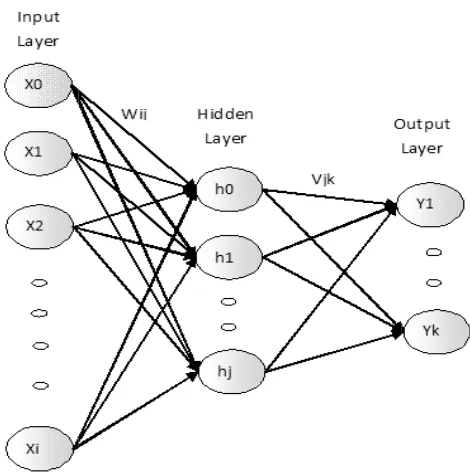
The network properties include connectivity (topology), type of
connections, the order of connections, and weight range. The topology of a neural
network refers to its framework as well as its interconnection scheme (Figure 2.2).
The framework is often specified by the number of layers and the number of
12
• The input layer: The nodes, which encode the instance presented to the network for processing
• The hidden layer: The nodes, which are not directly observable and hence hidden. They provide nonlinearities for the network.
• The Output layer: The nodes, which encode possible concept (or
value) to be assigned to the instance under consideration. For example
each input unit represents a class of object.
The behavior of a NN (Neural Network) depends on both the weights and
the input-output function (transfer function) that is specified for the units. The
ANN use variety of activation functions such as linear, logistic, hyperbolic tangent or
exponential functions etc. Some of the activation functions are explained below. This
function typically falls into one of three categories: linear, threshold, and sigmoid.
For linear units, the output activity is proportional to the total weighted
output. For threshold units, the output are set at one of two levels, depending on
whether the total input is greater than or less than some threshold value. For
sigmoid units, the output varies continuously but not linearly as the input changes.
Sigmoid units bear a greater resemblance to real neurons than do linear or
threshold units, but all three must be considered rough approximations. Logistics
function and hyperbolic tangent functions are the most common forms of sigmoid
functions used in ANN. It is advantageous to use because the relationship between the
value of the function at a point and the value of the derivative at a point reduces
computational burden during training. If the output range is between 0 and 1 then it is
called a binary sigmoid function or logistic function
The learning rule is one of the most important attributes to specify for a
neural network (Fu, 1994). Backpropagation is learning algorithm using
multilayer feedforward network with a different function in artificial neural. The
general multilayer feedforward network is fully interconnected hierarchy
consisting of an input layer, one or more hidden layer and output layer. During the
learning phase, input patterns are presented to the network in some sequences.
Figure 2.2 describes the process inside the feedforward backpropagation
x h Y W V B ( 2
xi : inpu hj : outp Yk : outp Wij : wei Vjk : wei
Basic Weight on Backpropag (Petterson, 1 1) Initiali a. Norm b. Ran c. Initi
2) Feed fo
a. Take
b. Acti
j
h
=
Figur
ut variable o put of node j put of node ight connect ight connect
c learning al
the netwo
ation learni
1996):
ization:
malization o
ndomize of w
alize of thre
forward step:
e training se
ive of input l
ij w
e
Σ+
=
1
1
re 22. Backp
of node i in i j in hidden l k in output l ing node i in ing node j in
lgorithm of b
ork so that
ing algorith
of input data
weight wij an
shold unit ac
: predicting T
t xi and tk
layer-hidden
i
jx …………
propagation N
input layer layer layer (predic n input layer n hidden laye
backpropaga
signal erro
hm can be
xi and targe
nd vjk using
ctivation, x0
T (with Y)
n layer unit w
………
Neural Netw
cted value of r and node j i er and node
ation modifie
or is minim
done step
et tk in form
(-1,1) value
0 = 1 and h0
with:
……… work
f node k) in hidden lay
k in output l
es the interco
mum (closer
by step a
of (0,1) rang
e = 1 ……… 13 yer layer onnection
r to zero).
as follows
ge
[image:33.612.202.437.78.316.2]14
c. Active of hidden layer-output layer units with:
j jkh v k
e
y
Σ+
=
1
1
……….. (II-2)
3) Minimize error of weight with vjk and wij adjustment. This process is called
backward step.
a. Computing error of the nodes in output layer (δk) to adjust vjk:
)
)(
1
(
k k k kk
=
y
−
t
t
−
y
δ
………...…. (II-3)j k old
jk new
jk
v
h
v
=
+
β
.
δ
. …..………..….…………. (II-4)Where:
β: constant of momentum
k
t : predicting value
b. Compute error of nodes in input layer (τj) to adjust weightswij:
)
.
)
1
(
j k k jkj
j
h
h
δ
v
τ
=
−
∑
... (II-5)jk j old
ij new
ij
w
v
w
=
+
β
.
τ
.
... (II-6)
4) Move to the next training set, and repeat step 2. Learning process is stopped
if yk are close enough to tk. The termination can be based on the error E. For
instance, learning process is stopped when E < 0.0001
∑
= = P P P tot E P E 1 1Where ( )
2 1 1 P k m k P k P y t
E =
∑
−=
……….. (II-7)
Where:
Tkp : target value of p-th data from training set node k yp : prediction value of p-th data from training set node k
The network can be used to predict t by inputting values of x after being
trained.
2.6.Accuracy Assessment
The most common accuracy assessment of classified remotely sensed data
is error matrix, sometimes known as confusion matrix. There are three types of
15 and user accuracy. Overall accuracy represents the number of correctly classified
pixels. The producer accuracy indicates the probability that a sampled point on the
map is that particular class. The user accuracy indicates the probability that a
certain reference class has also been labeled that class indicates (Janssen and
Huurneman 2001).
Error matrices are very effective representations of map accuracy, because
of the individual accuracies of each map category are plainly described along with
both errors of inclusion (commission error) and error of exclusion (omission
errors) present in the map and the error matrices can be used to compute overall
accuracy, producer’s and user accuracies, kappa coefficient. A commission error
occurs when an area is included in an incorrect category. An omission error
occurs when an area is excluded from the category to which it belongs. Overall
accuracy is simply the sum of the major diagonal (i.e., the correctly classified
pixels or samples) divided by the total number of pixels or samples in the error
matrix. This value is the most commonly reported accuracy assessment statistic.
Individual category accuracies instead of just the overall classification accuracy
are represented by producer’s and user accuracies.
An examination of the error matrix suggests at least two methods for
determining individual category accuracies. The most common and accepted
method is to divide the number of correctly classified samples of category X by
the number of category X samples in the reference data (column total for category
X). An alternate method is to divide the number of correctly classified samples of
category X by the total number of samples classified as category X (row total for
category X). It is important to understand that these two methods can result in
very different assessments of the accuracy of category X. It is also important to
understand the interpretation of each value. The mathematical example is shown
T S O P X Y Z 16
Table 2.4 Ex
Sum of the m
Overall Acc
Producer Ac
X = 28/30 =
Y = 15/30 =
Z = 20/40 =
Column To
xample of an
mayor diago
uracy = 63/1
ccuracy = 93% = 50% 50% X Y Z otal
n Error Matr
onal = 63
100 = 63%
User A
X = 28
Y = 15
Z = 2 Reference
X Y
28 14
1 15
1 1
30 30 rix
Accuracy
8/57 = 49%
5/21 = 71%
20/22 = 91% e Data
17
III. METHODOLOGY
3.1.Time and Location
Research is performed from September 2010 to March 2011. Step of data
collection, processing, analysis, and was done in campus Master of Science in
Information Technology for Natural Resources Management of Bogor
Agricultural University and National Coordinating Agency for Surveys and
Mapping
Seagrass conditions studied are located in Jakarta Province, Seribu Island
District, precisely in Pari Island. Geographically, it is situated between 05° 50′ -
05° 52′ South and 106° 34′ - 106° 38’ East. Study area in this research show in
[image:37.612.112.503.343.620.2]figure 3.1 below, covering Burung Island, Tengah Island, and Kongsi Island.
18
3.2. Material and Tools
The main data is satellite imagery and supporting data are digital map and
in-situ measurement data that obtained from survey. Whereas, the tools are
equipment, hardware and software, these are used for capturing, processing, and
analyzing the data.
3.2.1. Data Source
The principle supporting data for this study include the following discussed
matters:
1. Water condition data in 2009, data is acquisition from MODIS Aqua.
2. Satellite imagery of ALOS AVNIR-2 acquisition date September 18th,
2009, covering Pari Island and its surrounding. This spatial data provided
by National Coordinating Agency for Surveys and Mapping
(Bakosurtanal).
3. Landsat-7 acquisition year 2006, this satellite imagery provides by
Research Centre for Oceanography.
4. Field survey data, data is collected from visual observation and
measurement in the field directly in September 2010.
3.2.2. Required Tools
Several hardware and software’s and equipments that required in order
carrying out the whole research activities are:
1. Hardware consists of Notebook Intel ® Centrino Duo 1.83GHz, and
colour printer.
2. Software used are ENVI Image Processing, ESRI ArcView Spatial Analysis,
and MS Office 2007.
3. Equipment consist of Global Positioning System Garmin, and Scuba
equipment.
3.3.Research Step
There are three main steps to identifying seagrass condition. Firstly, image
pre-processing, secondly image classification, and last step is accuracy
19 applied before image classification, including subset and masking image. On
image classification stage, some data observation and measurement from field
survey directly were used for ANN classification, and another was used for
validation. Forty eight points of field data were divided into two data sets: 26 in
the training data set and 22 in the testing. Determination site observations and
field data capture technique is determined by random sampling at area (10m x
10m), adjusted with spatial resolution of ALOS AVNIR-2 satellite imagery. The
[image:39.612.98.504.268.727.2]research approach for seagrass identification in this study is shown in Figure 3.2.
20
3.3.1. Image Preprocessing
In the context of digital analysis of remotely sensed data, preprocessing
refer to those operations that are preliminary to the main analysis. Typically
preprocessing operations could include (1) radiometric preprocessing to adjust
digital values for the effect of hazy atmosphere and/or (2) geometric
preprocessing to bring an image into registration with a map or another image. In
this study, operation subset image that cover only study area, and masking land
objects that will not be classified was included as part of preprocessing process.
3.3.2. Image Classification
ALOS digital image processing was carried out using Environment for
Visualizing Images (ENVI) version 4.4. In this research, ANN supervised
classification was guided by variety of input data sets including field survey,
satellite imagery and expert knowledge to produce seagrass condition map.
Twenty two scenario processes would be done to compare the result of accuracy
as shown in Table 3.1.
The starting point of image classification is the different spectral
characteristics of the different materials on the Earth’s surface. Digital image
classification is the process of assigning pixels to classes. Usually each pixel is
treated as individual unit composed of values in several spectral bands. By
comparing pixels to one another and to those of known identity, it is possible to
assemble group of similar pixels into classes that match the informational
categories of interest to users of remotely sensed data. Field data were used to
determine training sites for three levels of seagrass cover classes ( ≤ 29,9%,
30-59,9%, ≥ 60% ) in the ANN supervised image classification process. Reflectance
signatures for each of the three different seagrass cover classes were extracted
from the ALOS AVNIR-2 scene of Pari Island for the calibration field sites,
which served as training sites for the image classification process. Characteristic
spectral reflectance signatures were defined for each of the target levels of
21 Table 3.1. Scenario Input Classification
Scenario Input
A 4 Original Band (Band 1, 2, 3, and 4) and water depth B 3 Original Band (Band 1, 2, and 3) and water depth C 3 Original Band (Band 1, 2, and 4) and water depth D 3 Original Band (Band 1, 3, and 4) and water depth E 3 Original Band (Band 2, 3, and 4) and water depth F 2 Original Band (Band 1 and 2) and water depth G 2 Original Band (Band 1 and 3) and water depth H 2 Original Band (Band 1 and 4) and water depth I 2 Original Band (Band 2 and 3) and water depth J 2 Original Band (Band 2 and 4) and water depth K 2 Original Band (Band 3 and 4) and water depth L 4 Original Band (Band 1, 2, 3, and 4)
M 3 Original Band (Band 1, 2, and 3) N 3 Original Band (Band 1, 2, and 4) O 3 Original Band (Band 1, 3, and 4) P 3 Original Band (Band 2, 3, and 4) Q 2 Original Band (Band 1 and 2) R 2 Original Band (Band 1 and 3) S 2 Original Band (Band 1 and 4) T 2 Original Band (Band 2 and 3) U 2 Original Band (Band 2 and 4) V 2 Original Band (Band 3 and 4)
The most important aspect in neural network is the training phase,
because the weights and the network characteristics are defined to be used to
another dataset. Before dataset used in training phase, it should be normalized in
range of 0 to 1, and then renormalized it after this phase. Dataset also has to be
splitting by randomize for the training and validation. Figure 3.3 show the
multilayer feedforward backpropagation neural network process that used in this
research.
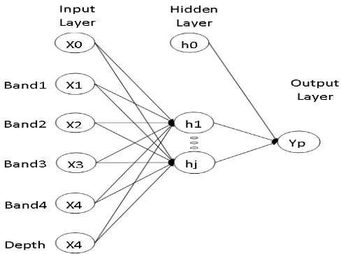
The number of nodes in the input layer depends on upon the number of
corresponding neural network. In this case 5 nodes for processing element of
inputs will be used to defined 3 possible output training pattern (i.e. seagrass
condition). There are three classes for seagrass condition; good, medium, and
poor. The three output pattern corresponds to the five inputs to generate the
22
Figure 3.3. Structure of Backpropagation Neural Network
The backpropagation learning is inclusive of supervise, which
determines the output from the input by using the training set. The training of
Artificial Neural Network has the following step based on ENVI help 4.4:
• Training Threshold Contribution field, enter a value from 0 to 1.0. The training threshold contribution determines the size of the contribution
of the internal weight with respect to the activation level of the node. It
is used to adjust the changes to a node's internal weight. The training
algorithm interactively adjusts the weights between nodes and
optionally the node thresholds to minimize the error between the output
layer and the desired response. Setting the Training Threshold
Contribution to zero does not adjust the node's internal weights.
Adjustments of the nodes internal weights could lead to better
classifications but too many weights could also lead to poor
generalizations.
• Training Rate field, enter a value from 0 to 1.0. The training rate determines the magnitude of the adjustment of the weights. A higher
rate will speed up the training, but will also increase the risk of
23 • Training Momentum field, enter a value from 0 to 1.0. Entering a
momentum rate greater than zero allows you to set a higher training rate
without oscillations. A higher momentum rate trains with larger steps
than a lower momentum rate. Its effect is to encourage weight changes
along the current direction.
• Training RMS Exit Criteria field, enter the value of RMS error at which
the training should stop. If the RMS error, as shown in the plot during
training, falls below the entered value, the training will stop, even if the
number of iterations has not been met. The classification will then be
executed.
• Training Iteration. The maximum iteration will decide at the practice.
The classification step of BPNN:
o Input layer of units, which are activated by the input image data. The
input image pixel values are linearly scaled to a value between 0.0 and
1.0 for input to the neural network with the minimum and maximum
image channel.
o Hidden layer is in between input layer and output layer. Calculate the
input hidden layer unit with Equation (II-4) and hidden
layer-output layer units with Equation (II-5).
o The output layer of units represents the output classes. In this study the
seagrass condition has 3 classes such as good (C1), medium (C2), and
poor (C3).
o Target is used for comparator the output. The target was obtained from
training area. Learning process is stopped if prediction values are close
[image:43.612.133.348.606.709.2]enough to the target value by calculating the error with equation (II-10).
24
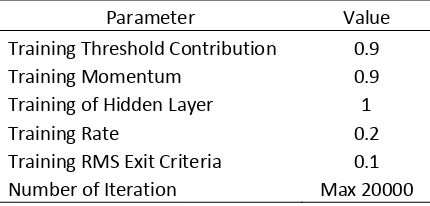
Table 3.2 shown neural network parameter used in this study, and
considering time consuming for all scenarios input have to be test, number
iteration set to maximum 20000.
3.3.3. Accuracy Assessment
After the classification has been completed, it is important to estimate the
accuracy of the result. The most common way to express classification accuracy is
the preparation of a so-called error matrix also known as confusion matrix or
contingency matrix. The columns of the matrix represent the verification data,
while the rows indicate the classified image. The elements of the matrix are the
number of pixels assigned to a class by the classification procedure, in
relationship with the identification through the verification data. Several
descriptive and analytical statistical techniques are based on the accuracy matrix.
The most common way to express the accuracy of such images/maps is by
a statement of the percentage of the map area that has been correctly classified
when compared with reference data or "ground truth." This statement is usually
derived from a tally of the correctness of the classification generated by sampling
the classified data, and expressed in the form of an error matrix .In this kind of
tally, the reference data (usually represented by the columns of the matrix) are
compared to the classified data (usually represented by the rows). The major
diagonal indicates the agreement between these two data sets. Overall accuracy
for a particular classified image/map is then calculated by dividing the sum of the
entries that form the major diagonal (i.e., the number of correct classifications) by
25 IV. RESULT AND DISCUSSIONS
4.1.General Condition
Pari Island waters are territorial waters that are surrounded by cliffs that
are protected from exposure to the open sea. This area has a water depth of 0
meters to 50 meters, with the shallow waters around the islands. Seagrass meadow
on Pari Island is the vegetation that lives in shallow waters. From the bathymetric
data obtained, it was found that the seagrass vegetation found in the data
collection is at a depth of 2 meters below the waters with a high brightness.
Seagrass in the island region is a region which rays are protected from exposure to
the high seas so that current flows in the region tend to be low even almost
non-existent (calm water), scattered seagrass vegetation in the region near the island
down to the bluff area.
A preliminary study in this research is recognizing water condition in
study area on September 2009 that used as reference for next remote sensing
process. Water clarity and Dissolved and Detritus Organic Matter from MODIS
satellite Imagery used as parameter to identify water condition (Figure 3.1). The
aim of this step is to avoid misinterpretation of the object for next image
processing. The diffuse attenuation coefficient at 490 nm (K490) is an indicator of
water clarity. K490 expresses how deeply visible light in the blue to green region
of the spectrum penetrates in the water column. The value of K490 represents the
rate at which light intensity at 490 nm is attenuated with depth. On September
2009, water clarity value is 0.04 (figure 4.1) which means water relatively clear,
because that light can penetrate in water column until 25 meters depth (0.04/1
meter).
Dissolved organic matter and particulate organic matter (or particulate
organic carbon, POC, defined below) is distinguished as the fractions of organic
matter in water samples that are either passed through or retained by a filter
(nominally a glass fiber filter with 0.7 µm pore size). Colored (also
called chromophoric) dissolved organic matter (CDOM) is optically detectable,
26
concentrations, CDOM will thus provide color to the water in which it is
dissolved. High concentrations of CDOM in ocean waters interfere with accurate
estimation of chlorophyll a concentration in remotely-sensed data. Figure 4.1
show the value of DOM is 0.009 gram/m3. It mean that water have low dissolved
organic matter. From the value of water clarity and DOM, generally it can be
[image:46.612.129.473.203.432.2]stated that water condition in Pari Island is good in September 2009.
Figure 4.1 Water Clarity and Dietrital Organic Matter in 2009
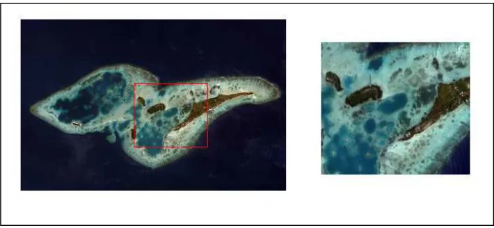
4.2. Image Preprocessing
An ALOS image (Figure 1), acquired on 18 September 2009, which is
used in this study is the result of image sensors AVNIR recording consisting of 4
channel / wavelength range. Channels 1, 2, and 3 respectively is the wavelength
range of blue (0.42 to 0.50 μm), green (0.52 to 0.60 μm), red (0.61 to 0.69 μm),
while channel 4 is the near infrared (0.76 to 0.89 μm) wavelength range. The
image used has a level 1B2, which was corrected in a systematic radiometric and
geometric. However, radiometric corrections remain to be done again because of
the shadow areas of digital value more than 0 (zero). From the histogram it can be
seen a minimum value of the digital image. This minimum value was used as a
deduction for the entire coverage of the image digital values. The result of
0.009677 0.044571429
0 0.01 0.02 0.03 0.04 0.05 0.06 0.07 0.08
Water Clarity
27 histogram adjustment for radiometric correction is presented in table 4.1. After
[image:47.612.132.386.145.229.2]performed histogram adjustment the minimum brightness value will be zero.
Table 4.1 Statistic before and after radiometric correction Basic
Statistics
Before After
Min Max Min Max
Band 1 131 219 0 93
Band 2 85 224 0 139
Band 3 53 184 0 131
Band 4 12 30 0 24
Afterward, even this image already geometrically corrected, ALOS image
2009 corrected again with Landsat-7 ETM satellite imagery 2006 which have
geometric corrected by theodolite water pass leveling, and registered to the UTM
Zone 48S, WGS84 coordinate system. Geometric correction intended to reduce
errors by position or location based on reference data that are considered true. In
order to correct geometric image, measuring the position of objects on the ground
are easily recognized among the ends of the pier, jeti, street intersection and
assumed that will not change for a long time. Eight control point used in this
image, because Pari Islands have flat topografi area. This Geometric correction
uses polynomial of control point type with linear order and nearest neighbor resampling. For medium resolution image on flat areas, the polynomials models
are sufficient. Total Root Mean Square (RMS) error in this geometric correction is
0.457151. This value describes how consistent the transformation is between the
different control points. The smaller RMS value indicated that accuracy of
geometric correction has improved. Overall, RMS error of less than 0.5 pixels was
achieved for each transformation.
After the radiometric and geometric have already done, it is better to
subset image that cover only study area. In these instances it is beneficial to
reduce the size of the image file to include only the area of interest (Figure 4.2).
This not only eliminates the extraneous data in the file, but it speed up processing
due the smaller amount of data to process.Subset images made to focus research
on areas of study and object of each pseudo color composite image and each
28
Figure 4.2 Subset of remote sensed data to focus at region of interest.
To avoid any interference from the influence of other objects, then the
image will be used for identification of seagrass condition, carried out restriction
area (cropping) or masking. Masking is mainly done to remove the clouds and
land objects that will not be classified. Masking method can be performed using
Boolean logic in the software and can also be done with manual digitization
processes. Separation of land and water objects intended for the spectral value
used in the classification process is not affected by the spectral value of the land.
To separate the land and waters will be determined boundary pixel value of land
and water (the value of landmarks). Values above the threshold (the value of
landmarks) will be considered null or no to that will appear is below the threshold
value.
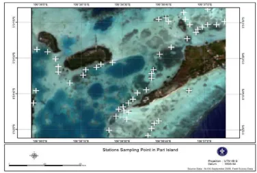
4.2.1. Field Survey
The field survey was carried out in four days (21, 22, 23 and 24 of
September 2010), one year after the acquisition of the ALOS image, but in the
same season based on visual observation. There are 48 (forty eight) sample point
area is recorded in the field by handheld Global Positioning System, mostly in
seagrass habitat (Figure 4.3). At each point, the percentage seagrass cover and
water depth was determined.
29 Figure 4.3. Field survey point with RGB 321 of ALOS
4.2.2. Region of Interest (ROIs)
Regions of interest (ROIs) are portions of images, either selected
graphically or selected by other means, such as thresholding. Typical uses of ROIs
include extracting statistics for classification, masking, and other functions. You
can use any combination of polygons, points, or vectors as an ROI. ROI
separability is option to computes the spectral separability between selected ROI
pairs for a given input file. Both the Jeffries-Matusita and Transformed
Divergence separability measures are reported. These values range from 0 to 2.0
and indicate how well the selected ROI pairs are statistically separate. Values
greater than 1.9 indicate that the ROI pairs have good separability. For ROI pairs
with lower separability values, you should attempt to improve the separability by
editing the ROIs or by selecting new ROIs. For ROI pairs with very low
separability values (less than 1), you might want to combine them into a single
30
In appendix B, it can be seen the separability of ROIs between good
seagrass and other habitat (poor seagrass, lagoon, sea, sand, coral, mix habitat,
and reef slope) are 2.0, except between good seagrass and medium seagrass is
1.99. The separability between medium seagrass and other habitat (poor seagrass,
lagoon, sea, sand, coral, mix habitat, and reef slope) are 1.93, 2.0, 2.0, 1.68, 1.88,
1.96 and 2.0 respectively. Value 2.00, 2.00, 2.00, 1.97, 1.95, and 2.00 are
achieved between poor seagrass and lagoon, sea, sand, coral, mix habitat, and reef
slope respectively. From that value of separability, two lower separability values
got between medium seagrass and sand (1.68), and medium seagrass and coral
(1.88). It can be stated, that not all the ROIs can well separability by this selected
point.
4.3.Image Classification
A classification scenario was developed to identify the seagrass condition
at Pari Island. For this purpose, shallow water habitat was classified into nine
classes; sea, sand, lagoon, coral, reef slope, mix habitat (coral, seagrass, seaweed,
and sand), poor seagrass, medium seagrass, and good seagrass. Those classes are
derived from field observation and considering by the spatial resolution of ALOS
data. The data set training areas are represented by each habitat type selected
based on the ground reference points collected from the field supported by the
local knowledge of the area. The image classification and mapping process were
done through supervised neural network classification.
During the classification process, RMS value and number of iteration
evaluated. It can be seen from plot of neural network (figure 4.4), that graph
begun stable from iteration 10000 during the classification which RMS value
approximately 0.65. Based on this plot, iteration 10000 was applied to all the
31 Figure 4.4. Plot of Neural Network Classification
Figure 4.5 ANN Habitat Classifications in Pari Island in 2010 (Scenario A)
Result of habitat classification as show in figure 4.5, poor seagrass
indicated by the blue color almost dominates the entire study. Mix habitat
(seaweed, coral, and seagrass) seen as yellow and sand (white color) also
dominant in Pari Island in 2010. Good seagrass (red) and medium seagrass (green)
[image:51.612.149.488.331.555.2]32
inputting al