Numerical modeling of the hydrodynamics of standing wave
and scouring in front of impermeable breakwaters
with different steepnesses
N. Tofany
a,n, M.F. Ahmad
b, A. Kartono
c, M. Mamat
d, H. Mohd-Lokman
aaInstitute of Oceanography and Environment (INOS), University Malaysia Terengganu, Malaysia bSchool of Ocean Engineering, University Malaysia Terengganu, Malaysia
c
Department of Physics, Faculty of Mathematics and Natural Sciences, Bogor Agricultural University (IPB), Indonesia d
Faculty of Informatics and Computing, University Sultan Zainal Abidin, Malaysia
a r t i c l e
i n f o
Article history:Received 21 October 2013 Accepted 22 June 2014
Keywords:
The RANS–VOF model Standing wave Steady streaming system Scouring pattern Breakwater steepness
a b s t r a c t
The aim of this paper is to numerically study the effects of breakwater steepness on the hydrodynamics of standing wave and scouring process in front of impermeable breakwaters. A two-dimensional hydrodynamics model based on the Reynolds Averaged Navier–Stokes (RANS) equations and the Volume of Fluid (VOF) method was developed and then combined with an empirical sediment transport model. Comparisons with an analytical solution and experimental data showed the present model is very accurate in predicting the near bottom velocity and capable of simulating the scour/deposition patterns consistent with experimental data. It was found that the additional terms of bottom shear stress in the momentum equations are necessary to produce a physical scouring pattern. Different breakwater steepnesses produce different characteristics of standing wave, the steady streaming system, and scouring pattern in front of the breakwaters, which also affects the correlations between them. An additional analysis of the turbulence field parameters and the sediment transport rate was also performed. All these important information will be presented in details in this paper and can be worthwhile for designing the breakwater in coastal areas.
&2014 Elsevier Ltd. All rights reserved.
1. Introduction
Improvement of the role of coastal areas in supporting human life has driven development of various breakwaters around the coast for protection. The breakwater dissipates the energy of the waves incoming to the beach through a series of wave transforma-tions for reducing their impact on the beach, especially during the storm conditions. The breakwater reflects a series incoming wave that impinges on it periodically. Then, the interactions of the incoming and reflected waves develop standing wave that consists of a series of nodes and antinodes in front of the breakwater. The standing wave on the surface produces the steady streaming, a system of recirculating cells below the surface (Tahersima et al., 2011; Yeganeh-Bakhtiary et al., 2010; Hajivalie et al., 2012). The steady streaming system is the key mechanism that is in charge for scouring in front of the breakwater.
One of the main concerns for coastal engineers in designing the breakwater is the stability. Local scour occurring in front of the breakwater is one of the main failure mechanisms (Sumer and
FredsØe, 2000). The presence of sediment erosion and undesired
deposition around the structure can threaten the breakwater stability and reduce its expected performance (Lee and Mizutani, 2008). Therefore, it is very important to understand the correla-tions between the characteristics of standing wave on the surface, the steady streaming system below it, and the scouring of sedi-ment at the bottom. A better understanding of these correlations is worthwhile for the engineers to better design the breakwater.
The significance of scouring has triggered many researchers to assess the scour pattern around coastal structures. de Best and
Bijker (1971) studied the problem of scouring of a sand bed in
front of a vertical breakwater, and found the scouring patterns were different forfine and coarse materials.Xie (1981)studied the scouring pattern in front of a vertical breakwater and found the different shape of scouring pattern was dependent not only on the sand grain size but also on the wave conditions. Two basic patterns proposed by Xie (1981)have been widely used as the benchmark for studying scouring in front of a vertical breakwater.
Irie and Nadaoka (1984), andHughes and Fowler (1991)conducted
Contents lists available atScienceDirect
journal homepage:www.elsevier.com/locate/oceaneng
Ocean Engineering
http://dx.doi.org/10.1016/j.oceaneng.2014.06.008
0029-8018/&2014 Elsevier Ltd. All rights reserved. n
Corresponding author at: Institute of Oceanography and Environment (INOS), University Malaysia Terengganu (UMT), 21030 Kuala Terengganu, Terengganu, Malaysia. Tel.:þ60176481408.
other experimental studies for vertical breakwater, Lee and
Mizutani (2008)for vertical submerged breakwaters,Sumer and
FredsØe (2000)for rubble-mound (sloped) breakwater, andSumer
et al. (2005)for low-crested rubble-mound breakwater.
The wave- structure–sediment interactions play an important role in the development of scour. To study these interactions, three approaches are generally used, namely, small-scale physical models, theoretical approaches, and numerical models. Each approach has its own advantages and drawbacks, so none is sufficient by itself. Physical models can provide insights into a realflow-field environment; however, in many situations such works produce incomplete results due to many limiting factors. The limits of the experimental works are such as the high experimental cost, various field meteorological conditions, drawbacks of measure-ment tools, difficulties in implementing physical parameters, scale effects, etc. An extensive number of successful empirical formulations are available in the literatures (e.g. Whitehouse,
1998; Sumer and FredsØe, 2002). However, the empirical
formula-tions cover only a limited number of wave condiformula-tions, setups, structure geometries, and sediment characteristics. These limits may lead to uncertainties and errors if they are used out of the range from which they are derived, which is a common problem faced in current design or pre-design conditions.
With the advancement of computer power today, the afore-mentioned limits are offset by developments and improvements of numerical models. Only the most recent numerical studies related to the present study are reviewed here.Gislason et al. (2009a,b)
used a 3-D Navier–Stokes solver, NS3, with the k-ω, SST (shear stress transport) model to calculateflow under the standing wave. Then, they combined the model with a morphological model consisting of the continuity equation for sediment (FredsØe and Deigaard, 1992) and the bed-load equation (Engelund and FredsØe, 1976). They simulated theflow of standing wave and the scouring pattern in front of the vertical and sloped breakwaters. However, the result was slightly inconsistent with the experimental data for the scour profile in front of the sloped breakwater.Hajivalie and
Yeganeh-Bakhtiary (2009)developed a numerical model
consist-ing of the RANS equation, VOF method, and the k-ε turbulence model. They studied only the effects of breakwater steepness on the hydrodynamics of standing wave and the recirculating cells patterns.Yeganeh-Bakhtiary et al. (2010)used the same model to study the hydrodynamics of standing wave in front of a vertical breakwater. They focused on studying the effects of wave over-topping on the hydrodynamics of a standing wave, recirculating cells, and turbulencefield. Then,Tahersima et al. (2011)coupled the hydrodynamics model ofYeganeh-Bakhtiary et al. (2010)with sediment transport formulae (Engelund and FredsØe, 1976; Bijker, 1971) and a bed profile change model (FredsØe and Deigaard, 1992) to study scouring in front of a vertical breakwater. They numerically showed the scouring patterns under the case of overtopping and without overtopping. However, the resulted patterns did not follow the scouring pattern ofXie (1981).
The above experimental and numerical studies have studied the hydrodynamics of standing wave and scouring pattern under the effects of four different factors. They are the wave conditions, breakwater shape, sediment grain size, and overtopping occur-rence. Various numerical simulations have given more attention on the hydrodynamics of standing waves in front of the vertical/ sloped breakwater. Only some of these studies extended the analysis by including the scouring at the bottom (Tahersima et al., 2011; Gislason et al., 2009a,b). However, these studies did not produce satisfying results. In addition, the experimental study for sloped breakwater (Sumer and FredsØe, 2000; Sumer et al., 2005) only provides limited descriptions on the important physi-cal aspects. They are the characteristics of standing wave, the steady streaming system, and sediment transport process. In fact,
a detailed description of such aspects is necessary to understand the effects of breakwater steepness on the correlations between them. Therefore, this paper is focusing to discuss more deeply the effects of breakwater steepness on the characteristics of standing wave, steady streaming system, and, in particular, scour-ing pattern.
The present model combines the RANS equations, VOF method, ak-εturbulence closure model, and an empirical sediment trans-port formula of Bailard (1981). The model includes additional terms of bottom shear stress as used byKarambas (1998)in the momentum equations. As using the Bailard's formula, prior tests showed the terms of bottom shear stress are necessary to produce a physical scouring pattern. None of the RANS-based numerical models (Hajivalie and Yeganeh-Bakhtiary, 2009; Yeganeh-Bakhtiary et al., 2010; Tahersima et al., 2011) have taken these terms into their models. In addition, none of the previous scouring simulations (Tahersima et al., 2011; Gislason et al., 2009a,b) used the Baillard's formula. In this paper, it will be shown that the scouring patterns simulated by the present model are more consistent with the experimental results (Xie, 1981; Sumer et al., 2005) than the previous studies.
2. The numerical model
The present model used the SOLA-VOF code (Nichols et al., 1980) as the basic platform. However, some modifications and additional features were added into the code in order to make it more appropriate for simulating the interactions between wave, structure and sediment. This section presents the main compo-nents of the present model.
2.1. Governing equations offluidflow
νt¼Cd k2
ε; ð7Þ
wheretis time,uandvare the mean velocity components in thex
and y directions, respectively, p is the mean pressure, g is the gravity acceleration, ρ is the density of the fluid, ν and νt are respectively the fluid and eddy viscosities, k is the turbulence kinetic energy,Pris the production of turbulence kinetic energy,
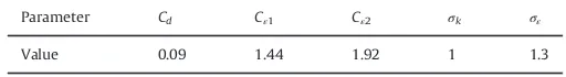
εis the turbulence dissipation rate,θis the partial cell treatment parameters,τbxandτbyare the bottom shear stresses. The model constants were set according to Launder and Spalding (1974)
and are presented in Table 1. The bottom shear stresses were estimated fromKarambas (1998):
τbx
whereubandvbare the horizontal and vertical components of the
near bottom velocity, andfwis the friction coefficient.
2.2. Cross-shore sediment transport model
An empirical transport formula (Bailard, 1981) was used to calculate the transport rate of sediment at the bottom. In this model, particles were assumed as non-cohesive. The Bailard's formula adapted the Bagnold's energetic approach (Bagnold, 1946) that separated the efficiency factors between bed-load and suspended load transport modes. The formula of total volumetric sediment transport rate,S(t), is as follows:
SðtÞ
Here,Sb(t) andSs(t) are the instantaneous volumetric sediment transport rate for bed-load and suspended load, respectively,ρsis the density of sediment,wis the fall velocity of sediment,εbandεs are the bed-load and suspended-load efficiency factors, respec-tively, cf is the drag coefficient of the bed, p is the sediment porosity,φis the angle of repose,αis the bed-slope angle,ub(t) is the instantaneous near bottom fluid velocity, and o 4 is for time-average;Table 2presents the parameters which are used in the current simulation. In the Bailard's original equation, it was recommended to use a value ofcf¼0.005. While in the present work, 0.5fwwas used to replacecf, in which the skin friction factor,
fw, was formulated based onJonsson (1966)as follows:
fw¼exp 5:213
whereris the bed roughness that is assumed as equal toD50, and
aois the amplitude of orbital motion at the bottom, for thefirst order linear wave theory:
ao¼ H
2 sinhð2πd=LÞ; ð13Þ
where His the incident wave height, dis the water depth, and Lis the wavelength. The change of bed profile was calculated by the continuity equation for sediment, according toFredsØe and Deigaard (1992)as follows:
whereyis the bed level andpis the porosity of sediment.
3. Numerical solutions
3.1. Boundary conditions
The free surface motion was solved with the Volume of Fluid (VOF) method (Hirt and Nichols, 1981). With the VOF-method, the kinematic and dynamic boundary conditions at the free surface are satisfied. The solution of the volume fraction of fluid, F, was obtained by solving the following conservation equation:
∂θF
The Dirichlet-type boundary condition was used at the left boundary to generate the wave into the numerical domain. In addition, to reduce the intermixing of the generated and unphy-sical reflected waves at this boundary, the weakly reflecting boundary condition, proposed byPetit et al. (1994)was applied. It is formulated as follows:
∂φ
whereφiis the variables of incident wave signals andφis for the computed variables, including the free surface displacement and velocities. The partial cell treatment technique of NASA-VOF2D code (Torrey et al., 1985) was adopted to create the breakwater structure on the right of numerical domain.
At the bottom and along the solid boundary of the breakwater structure, for simplicity, free-slip rigid wall was taken as the boundary conditions.
ui;1¼ui;2; vi;1¼0; ki;1¼ki;2; εi;1¼εi;2; ð17Þ
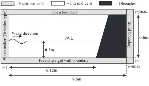
Although it is important, in the present model the effects of the boundary layer at the bottom and along the solid boundary were neglected. Nevertheless, it will be shown inSection 4.1, the present model can produce better scouring patterns than the previous models (Tahersima et al., 2011; Gislason et al., 2009a,b), whereas they included the detailed description of the boundary layer at the bottom. At the top, an open boundary condition was applied.Fig. 1depicts the computational domain that was used for numerical experiments, in which the results of these experiments will be presented inSection 4.2.
The turbulence boundary conditions at the free surface were assumed with zero verticalfluxes ofkandε:
∂k
∂n¼0; ∂ε
∂n¼0 ð18Þ
Table 1
Constants of thek-εturbulence closure model (Launder and Spalding, 1974).
The Neumann continuative boundary condition was defined at the left and top boundaries:
∂k
The calculation starts from zero velocity and hydrostatic pressure for fluid field, and aflat bed profile was initialized at y¼0 cm at the bottom. The initial conditions for the turbulence field were set according toLin and Liu (1998)andBakhtyar et al. (2009)as follows: empirical coefficient as given inTable 1.
3.3. Numerical schemes
From Eqs. (1)–(7) and (15), six unknown variables must be solved, includingu, v, p, F,k, andε. Thefinite difference method was employed to solve all these partial differential equations. The time evolution of the unknown variables was advanced based on the Simple Implicit Method for Pressure-Linked Equations (SIMPLE) algorithm, firstly proposed by Patankar (1980). The procedure of this algorithm for one computational cycle can be presented step by step as follows:
1. The velocity components were approximated using Eqs. (2)
and (3) by neglecting the effects of pressure change. In this
step, the values of bottom shear stresses were taken from the previous time-step. The advection terms of these equations were discretized using a combination of thefirst order upwind-central differencing scheme, while the diffusion terms were discretized using the second order central-differencing scheme. 2. The pressure field was updated by iteratively adjusting the approximated velocity components until satisfying the conti-nuity equation, Eq.(1). The Successive Over Relaxation (SOR) method was used for this purpose.
3. The new velocity values were updated by including the effects of pressure change. Then, the new bottom shear stress values in Eq.(8)were computed using the updated bottom velocities as input. These values were used for the next computational cycle. 4. The turbulence field componentsk,ε, andνt were computed using Eqs. (4)–(7). The discretization was done using the similar schemes as in the step (1).
5. The newF-value for each cell was updated based on the donor– acceptor algorithm and then the new free surface configuration was reconstructed using the newF-values.
6. The boundary conditions were applied in each step above. 7. The transport rate of sediment was calculated using Eqs.(9)–(11),
and then the new bed profile was calculated using Eq.(14). Then a new cycle was done by repeating all these steps. The cycles were repeated until the end of computational time was exceeded.
3.4. Stability of the numerical scheme
To ensure the stability of computation, in every cycle the value of∆t was adjusted to satisfy the following criterions (Bakhtyar
et al., 2009):
1. Thefluid cannot travel more than one computational cell in each time-step:
2. Momentum must not diffuse more than approximately one cell in one time-step:
3. Surface waves cannot travel more than one cell in each time-step:
whered(m) is the water depth.
4. The relative variations of k and ε in a time step should be significantly less than unity:
Δtrmin k
The code of the present model, processing, visualization, and interpretation of the computed results were all written and performed using MATLAB R2013a-64 bits in a personal computer with processor of Intel (R) Core (TM) i5-3230 M [email protected] GHz, installed memory (RAM) of 16.0 GB, and 64-bit operating system of Windows 7.
4. Results and analysis
4.1. Model validation
Accuracy of the sediment transport prediction is highly depen-dent on the predicted values of near-bottom horizontal velocity, especially under the locations of node and halfway between node and antinode, orL/4 and L/8 from the breakwater, respectively. These are where the velocity is highly varied. The near-bottom horizontal velocity is the most important parameter as the main input for the Bailard's formula. The present model was validated by comparing the numerical results with an analytical solution of standing wave and experimental data of Xie (1981) and Zhang et al. (2001)for the near-bottom horizontal velocity. To strengthen the validity of numerical results, 14 different tests were performed with parameters ranging from 0.01 to 0.67 for the wave steepness and 0.05–0.24 for the relative depth in three different water depths of 0.3 m, 0.5 m, and 0.65 m. Three of these tests were 0.3m
Free slip rigid wall boundary Wave direction
SWL
Solid boundary
= Fictitious cells = Internal cells = Obstacles
i=1 i=imax
j=1 j=jmax
based on the experiment ofZhang et al. (2001)and performed by including the overtopping process; seeTable 3for the complete parameters andFig. 2for the computational domains, which are according to the experiments ofXie (1981)andZhang et al. (2001). In addition, the results were also compared to an analytical solution of standing wave based on the second order theory of Miche as follows:
uðx;y;tÞ ¼2πH T
coshkðyþhÞ
sinhkh cos kxcos ωt
þ3π
2H2 2TL
cosh2kðyþhÞ
sinh4kh sin 2kxsin 2ωt; ð26Þ where k¼2π/L, ω¼2π/T, x and y are horizontal and vertical coordinates, andtis time.
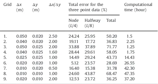
Prior to the fourteen tests inTable 3, nine tests were performed by varying the grid size tofind the best grid size. The same wave parameters and duration were set for all the tests. They were taken from Test 2 inTable 3for 10 T long duration.Table 4presents the tested grid sizes and the results in terms of the errors produced and the computational time required by each grid size. Eventhough, it did not produce the smallest total error, Grid 2 was decided as the grid for all simulations inTable 3, and it was not Grid 6 that produced the smallest total error (28.69%). This choice was made by considering that the errors under the node
and the halfway of Grid 2 were more proportional than the errors of Grid 6. Even the accuracy under the halfway was better than Grid 6. In fact, the areas between the node and antinode are very important because they are the locations in which the most intense sediment movement occurs. Grid 7 was not decided because, when compared to Grid 2, it took a very long Table 3
Experimental conditions for validation.
Experiment Flume Test d(m) H(m) T(s) L(m) d/L H/L hwall Overtop
Xie (1981) Small 1 0.3 0.050 2.41 4 0.075 0.013 1 No
2 0.3 0.065 1.53 2.4 0.125 0.027 1 No
3 0.3 0.057 1.86 3 0.100 0.019 1 No
4 0.3 0.06 3.56 6 0.050 0.010 1 No
5 0.3 0.050 1.17 1.71 0.175 0.029 1 No
6 0.3 0.057 1.32 2 0.150 0.029 1 No
Large 7 0.5 0.050 1.7 3.33 0.150 0.015 1.2 No
8 0.5 0.075 3.12 6.67 0.075 0.011 1.2 No
9 0.5 0.100 3.12 6.67 0.075 0.015 1.2 No
10 0.5 0.060 1.7 3.33 0.150 0.018 1.2 No
Zhang et al. (2001) 11 0.65 0.090 1.4 2.7 0.241 0.033 0.75 Yes
12 0.65 0.120 1.4 2.7 0.241 0.044 0.75 Yes
13 0.65 0.150 1.4 2.7 0.241 0.056 0.75 Yes
14 0.65 0.180 1.4 2.7 0.241 0.067 0.75 Yes
Wave maker
1m
L/4
L/8
0.45m 0.30m
6m 14m
11m 20m
1.2m 0.65m 0.50m
L/4 L/8
Wave maker
L/4
0.65m
5.4m
0.75m
Wave maker
Fig. 2.Computational domains for the validation of the horizontal near bottom velocity. (a) Theflume ofZhang et al. (2001), (b) the smallflume of the experiment ofXie
(1981), and (c) the largeflume of the experiment ofXie (1981); the red lines represent the cross sections for measurement of horizontal velocity data. (For interpretation of the references to color in thisfigure legend, the reader is referred to the web version of this article.)
Table 4
The results of the grid convergence test. Wave parameters¼Test 2 inTable 3. Duration¼10 T.
Grid Δx (m)
Δy (m)
Δx/∆y Total error for the three point data (%)
Computational time (hour)
Node (L/4)
Halfway (L/8)
Total
computational time, which was nineteen times longer, to improve the accuracy of only around 5%.
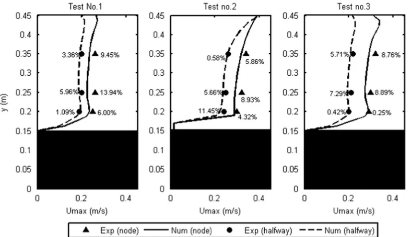
Fig. 3shows the comparisons between the numerical results
and experimental data ofXie (1981)for the maximum horizontal velocities of three different wave conditions, namely, Test 1, Test 2, and Test 3 in Table 3. The experimental data were collected at three different depths under the node (x¼L/4) and the halfway (x¼L/8), as shown in Fig. 2. The numerical results are very closed and consistent with the experimental data, in which the highest magnitude of Umax is located near the surface that subsequently reduced towards the bottom, and the velocity magnitude at the node is always greater than at the halfway.
Fig. 3also shows that the predicted velocities under the halfway are more accurate than the predicted velocity under the node. Eventhough there are slight errors, however, these errors are still reasonable and do not obscure the meaning of main physical process being simulated.
Fig. 4 shows the comparisons of the maximum horizontal
velocities (Umax) near the bottom for the fourteen tests as given inTable 3,Fig. 4(a) and (c) for the numerical results vs. analytical solutions, while Fig. 4(b) and (d) for the numerical results vs. experimental measurements.Fig. 4(a) and (b) shows the values of Umax measured at thefirst node of standing wave (x¼L/4), while
Fig. 4(c) and (d) for the Umax values measured at the halfway
between thefirst node and antinode of standing wave (x¼L/8). In the experiment ofXie (1981), theUmaxvelocities were measured at y¼0.03 m from the bottom for Test 2, Test 6 and Test 5, while at y¼0.05 m for the other 7 tests. In the experiment ofZhang et al. (2001), theUmaxvalues were measured at the red point as shown inFig. 2, which is 0.25 m above the bottom under the location of thefirst node of standing wave (x¼L/4).
In each data set, a linear regression line is plotted, and then the relative error, the equation of line,R2-value, and correlation
coefficient (A) are also presented to measure the strength of a linear relationship between the compared variables. The values of coefficient correlation in all these figures are higher than 0.9, A¼0.910 forFig. 4(a), A¼0.918 for Fig. 4(b), A¼0.972 for
Fig. 4(c), and A¼0.973 for Fig. 4(d). These results show that the numerical results are in a very good agreement either with the
experimental data or with the theoretical results, in which the numerical results at the halfway has a better accuracy than at the node.
4.2. Validation of the scour/deposition pattern
Two qualitative comparisons were conducted to validate cap-ability of the present model in simulating the scour/deposition pattern. In thefirst comparison, the present model was compared with the experimental data of Sumer et al. (2005) and the numerical results of Gislason et al. (2009a,b). The experimental results ofSumer et al. (2005),Fig. 6(a) and (b), are used as two reference cases.Sumer et al. (2005) conducted the experiment using regular waves for a vertical breakwater and a rubble mound breakwater with a slope of 1:1.5 in a waveflume, 0.6 m in width, 0.8 m in depth and 28 m in length. The test conditions of the experiment are summarized in Table 5, while the sediment properties are the same as presented in Table 2. It has been analyzed by Sumer et al. (2005), the sediment material as in
Table 2is falling into the category of coarse material, in which the bed load with no suspension is the main mode of transport. It means that, similar to the scour pattern of Xie (1981) for the coarse material (Fig. 5), the scour occurs under the halfway, while the deposition under the node of standing wave. It can be observed inFig. 6(a) and (b) that the scour/deposition pattern in front of the vertical and sloped (rubble-mound) breakwaters generally can be differentiated as follows:
1. Considerable scour occurs at the toe in the case of sloped breakwater, (Fig. 6(b)) in contrast to zero scour in the case of vertical breakwater (Fig. 6(a)).
2. The precise location of the maximum deposition is shifted in the onshore direction in the case of sloped breakwater. 3. The maximum scour depth in front of the sloped breakwater is
about 25% smaller than in the case of vertical breakwater.
The present model and numerical simulations ofGislason et al.
(2009a,b)used the same test conditions and sediment
character-istics as in the experiment ofSumer et al. (2005). In the vertical
Fig. 3.Comparison of numerical results and experimental data (Xie, 1981) for the maximum horizontal velocity. Wave parameters¼Test 1, Test 2, and Test 3 inTable 3.
breakwater case, shown inFig. 6(c) and (e), both models simulated the scour/deposition patterns, which are consistent with the experimental results. Although Gislason et al. (2009a,b) have included the effect of boundary layer at the bottom in their model; the scour/deposition profile in the case of sloped breakwater
(Fig. 6(f)) is apparently not consistent with the experimental
result. Meanwhile, in the sloped breakwater case, the present model produces the scour/deposition pattern (Fig. 6(d)), which is highly consistent with the experiment (Fig. 6(b)) in terms of the locations of scour troughs and deposition ridges.
In addition, the present model can show all the three different characteristics of scour/deposition pattern between the vertical and sloped breakwaters as presented above. The patterns of the present model (Fig. 6(c) and (d)) are only different to the experi-ment (Fig. 6(a) and (b)) in terms of the sizes of scour/deposition depth and width, which generally are smaller. It is due to the patterns in Fig. 6(c) and (d) are not the equilibrium profiles, produced after 10 T (or 20 s), and while the experimental results are produced in the equilibrium state reached after 1200 T (or 40 h).
In the second comparison, the present model was compared to the numerical simulation of Tahersima et al. (2011). The test conditions for this comparison (given inTable 6) were taken from the experiment of (Xie, 1981, experiment no. 11a, Table 1, page 8). The scour/deposition patterns of the both models are presented in
Fig. 7, in which thex-axis is normalized by the wavelength (L). The experiment observed that the type of scouring pattern of this test condition is categorized as coarse material (Xie, 1981, Table 11, page 20). As shown in Fig. 7(a), the scour/deposition pattern of
Tahersima et al. (2011)is quite misleading, not following the Xie's pattern for coarse material (Fig. 5). Meanwhile, the scour/deposi-tion pattern of the present model (Fig. 7(b)) is accurately similar to the Xie's pattern for coarse material (Fig. 5). The scour troughs are located under the halfway (L/8 from the breakwater) and the deposition ridges occur under the node (L/4 from the breakwater) of standing wave.
The two comparisons above have shown the capability of the present model in simulating the scour/deposition patterns in front of the vertical and sloped breakwaters. Although, the bed profiles are not in the equilibrium state, the locations of scour troughs and deposition ridges are highly consistent with the experimental
Fig. 4.Comparison of maximum horizontal-velocities near the bottom: (a) numerical vs. theoretical at the 1st node (x¼L/4), (b) numerical vs. experimental at the 1st node
(x¼L/4), (c) numerical vs. theoretical atx¼L/8,and (d) numerical vs. experimental atx¼L/8. Wave parameters are given inTable 3. Grid size¼Grid 2 inTable 4.
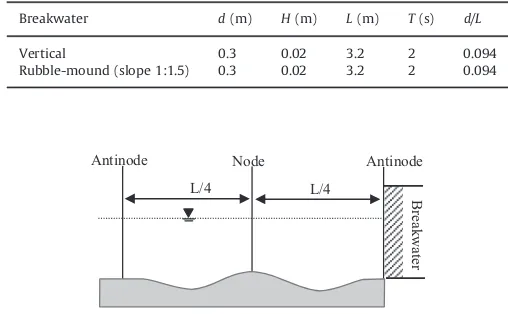
Table 5
Test conditions for the validation of scour/deposition pattern in thefirst compa-rison case.
Breakwater d(m) H(m) L(m) T(s) d/L
Vertical 0.3 0.02 3.2 2 0.094
Rubble-mound (slope 1:1.5) 0.3 0.02 3.2 2 0.094
L/4 L/4
Node Antinode Antinode
Breakwater
patterns (Sumer et al., 2005; Xie, 1981), showing better results than the previous numerical simulations (Gislason et al., 2009a,b;
Tahersima et al., 2011). An additional test (using the physical
conditions in Table 6) found that, when applying the Bailard's formula, the additional terms of bottom shear stress are required in the momentum equations to produce physical bed profile. Without these terms, the present model produced an unphysical bed profile as shown inFig. 7(c)
4.3. Numerical experiments of the breakwater steepness effects.
The change of bed profile in front of the breakwater is the manifestation of complex interactions between the wave, break-water, and sediment. Differences of the scour/deposition patterns in front of the two different breakwaters (as observed in the experiment ofSumer et al. (2005)) indicate that these interactions become changed due to the slope of the breakwater. The
characteristics of standing wave and steady streaming system are the most important features to analyze the effects of break-water steepness on the scour/deposition pattern at the bottom.
In order to study more deeply the effects of breakwater steepness, five different simulations for different breakwater steepnesses were performed in the same physical conditions. The parameters of the simulation are presented in Table 7. All simulations were performed for 20 s long duration or equal to 10 wave periods. The computational domain is presented in Fig. 1
with size of 8.5 m in length and 0.6 m in height. The regular sinusoidal waves were generated in the domain using the Dirichlet-type wave generator, which is located at the left bound-ary (6.12 m away from the toe of the breakwater). Based on the grid convergence test, the numerical domain was discretized using Grid 2 inTable 4for all simulations. The characteristics of standing wave, steady streaming system, and scouring/deposition pattern in each case were analyzed and the results are presented here. In addition, the analysis of turbulencefield parameters and sediment transport rate are also presented.
Figs. 8 and 9illustrate the snapshots of free surface motion and velocity vectors for the vertical and the 1:2-sloped breakwater cases, respectively. After the first incoming wave impacts the breakwater, interaction between the reflected and second incident waves starts to develop fully standing waves in front of the vertical breakwater. The 1:2-sloped breakwater has a different reflecting coefficient to the vertical breakwater. Consequently, it changes the Node Antinode Node Antinode
L/4 L/4 L/4
0 0.5 1.0 1.5 x(m)
0 1
2
Antinode Node Antinode Node
L/4 L/4 L/4
0 0 1
2
0.5
1.0
S(cm) x(m)
L/4 L/4
L/4
Node Antinode Node Antinode
a) b)
2.0cm 1.5
0.5 1.0
0.0 0.5 1.0 1.5 2.0
Breakwater x
0.5 1cm
0
-0.5
-1
-1.5
-2 Node Antinode Node
L/4 L/4
b) a)
Fig. 6.Scour/deposition patterns. The experiments ofSumer et al. (2005)–equilibrium state: (a) vertical and (b) slope 1:1.5. The present model–no equilibrium state
(duration: 10 T): (c) vertical and (d) slope 1:1.5. The numerical results ofGislason et al. (2009a,b)–equilibrium state: (e) vertical and (f) slope 1:1.5 (thick line: numerical simulation and thin line (with ripples): the raw data of experimental results inFig. 6(a) and (b)).
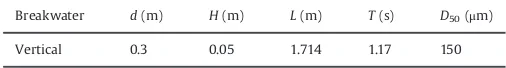
Table 6
Test conditions for the validation of scour/deposition pattern in the second compa-rison case.
Breakwater d(m) H(m) L(m) T(s) D50(μm)
interaction of incident and reflected waves in front of the break-water. The sloping part of the breakwater gives a space for the wave to run-up over the slope and then run-down after it reaches the maximum run-up distance. During this event, part of the wave energy is dissipated and another part is transformed to generate turbulence in the meanflow (as will be shown later). Hence the reflected wave becomes weaker than in the case of vertical breakwater, in which almost all the energy of the incident wave is reflected back by the vertical breakwater.
As the result, the partially standing wave is developed in front of the 1:2-sloped breakwater. It is expected that under the action Tahersima et al. (2011)
-0.25 0.00 -0.50
-0.75 -1.00
-2.0 -1.5 -1.0 -0.5 0.0 0.5 1.0 1.5 2.0
X/L
Zi (cm)
100% 80% 40% 10%
Vertical breakwater
Fig. 7.Scour/deposition patterns: (a) the numerical simulations ofTahersima et al. (2011)–equilibrium state, (b) the present model–no equilibrium state (duration: 10 T)
and (c) the present model without bottom shear stress calculation.
Table 7
Parameters of numerical experiments.
Test no. d(m) H(m) L(m) T(s) d/L Slope Steepness
1. 0.3 0.02 3.2 2 0.094 Vertical – 2. 0.3 0.02 3.2 2 0.094 1:1.2 Steep 3. 0.3 0.02 3.2 2 0.094 1:1.5 Steep 4. 0.3 0.02 3.2 2 0.094 1:2 Gentle 5. 0.3 0.02 3.2 2 0.094 1:4 Very gentle
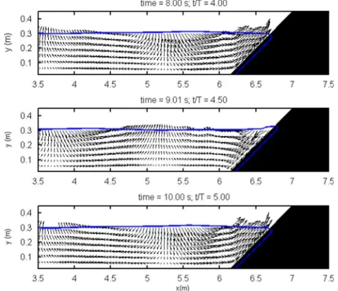
Fig. 8.Snapshots of free surface motion and velocity vectors of standing wave in
front of the vertical breakwater.
Fig. 9. Snapshots of free surface motion and velocity vectors of standing wave in
of partially standing wave, theflow conditions below the surface will be changed and weaker than in the case of fully standing wave, which eventually reducing the sizes of scour depth and deposition height at the bottom. Different steepnesses of the breakwater will produce different characteristics of partially standing wave, flow condition, and scour/deposition pattern at
the bottom. All these features will be discussed systematically in the next paragraphs.
Fig. 10shows the free surface profile of standing wave in the five breakwater cases as the water surface attain its maximum and minimum extreme positions. The standing wave that consists of a series of nodes and antinodes is formed in front of the five breakwaters. Different characteristics of the standing wave are observed in each case. Firstly, the extreme positions of water surface in each case are reached at different times. These positions occur twice in every wave period. The sloped breakwater induces a time lag in reaching these extreme positions; in which the time lag is increased when the slope becomes gentler. For instance, the extreme positions of water surface depicted in Fig. 10(a) are reached at 4 T, 4.5 T, 5 T, 5.5 T,…, 9 T, and 9.5 T, in Fig. 10(b)
at 4.05 T, 4.55 T, 5.05 T, 5.55 T,…, 9.05 T, and 9.55 T, while in Fig. 10(c) at 4.10 T, 4.6 T, 5.1 T, 5.6 T,…, 9.1 T, and 9.6 T. Longer time
lag was observed in the 1:2 and 1:4-sloped breakwater cases. The resulted time lag indicates that there is a phase change in the development of standing wave due to different breakwater steepnesses.
Secondly, the shape of standing wave in front of the vertical breakwater (Fig. 10(a)) is relatively more symmetric. This symme-trical feature starts to change in the cases of sloped breakwater, especially in the area over the slope. Thirdly, in general, in the cases of sloped breakwater, the 1st antinode is located over the slope and the locations of 1st node and 2nd antinode are shifted to the onshore direction, getting closer to the location of the break-water's toe. Even there are a 1st node and 2nd antinode that form over the slope, as in the case of 1:4-sloped breakwater (Fig. 10(e)). Fourthly, the resultant amplitude of the standing wave is reduced when the breakwater steepness becomes gentler;Fig. 10(e) clearly shows this feature. All these results have direct effects to the steady streaming system and the scour/deposition pattern at the bottom.
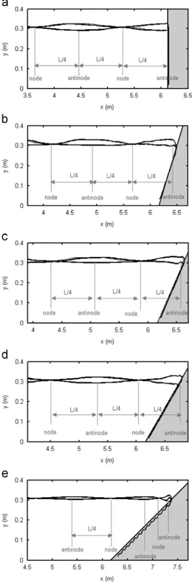
As the consequence of different standing wave characteristics, the scour/deposition pattern at the bottom is formed differently in front of each breakwater. Fig. 11 shows the scour/deposition pattern in each of breakwater case, which is developed after 10 T. As presented inSection 4.2, the sediment material used in the present experiment is falling into the category of coarse material with bed-load and no suspension mode as the dominant transport mechanism. The scour/deposition pattern in front of the vertical breakwater (Fig. 11(a), which is similar toFig. 6(c)) follows accurately the scour/deposition pattern of Xie (1981)for coarse material (Fig. 5). Correlations between the standing wave on the surface and the scour/deposition pattern at the bottom can be more clearly seen by relatingFigs. 10 and 11. Locations of node and antinode in Fig. 11 are referring to Fig. 10. Information of the locations of node and antinode plays an important role in facil-itating analysis of steady streaming system and scour/deposition pattern at the bottom. The present model can give a good presentation for such locations.
In analyzing the breakwater steepness effects on the scour/ deposition pattern, the steepness of the breakwater is classified into three categories: steep, gentle, and very gentle (seeTable 7). The pattern in the case of the vertical breakwater is used as the reference case for the other breakwaters. It must be noted that the scour/deposition patterns of Fig. 11(a) and (c) are equal to
Fig. 6(c) and (d), respectively. The scour/deposition patterns in front of the steep and gentle breakwaters (Fig. 11(b), (c), and (d)) generally are still in the form of alternating between scour troughs and deposition ridges. However, several differences are observed and can be drawn as follows:
1. Although substantial scour occurs in front of the vertical breakwater, there is no scour at the toe of the breakwater. In
Fig. 10.Free surface profile of the standing wave in front of thefive breakwater
contrast, scour occurs at the toe of the breakwater in the case of 1:1.2 (Fig. 11(b)) and 1:1.5 (Fig. 11(c)) sloped breakwaters. While in the case of 1:2 sloped breakwater (Fig. 11(d)), instead
of scour, deposition is formed in front of the toe of the breakwater.
2. The sizes of scour troughs and deposition ridges in the case of sloped breakwaters are generally smaller than in the case of vertical breakwater. In general, the sizes are decreased when the breakwater steepness becomes gentler.
3. The locations of scour troughs and deposition ridges in the case of sloped breakwaters move closer to the breakwater. This is according to the shifting of node and antinode locations due to the different steepnesses. More gentle the slope, the locations become closer to the breakwater.
4. The precise location of the maximum deposition ridge that closest to the breakwater is shifted, not exactly under the node. It is shifted to offshore direction in the case of 1:1.2-sloped breakwater, while it is shifted to the onshore direction in the cases of 1:1.5 and 1:2-sloped breakwaters.
5. Scour occurs under the location of antinode in the case of gentle slope (1:2) breakwater (Fig. 11(d)), while in the cases of vertical and steep slope breakwaters there is no scour at such location.
6. The bed profile in the case of very gentle slope (1:4) breakwater is almost not changed. Different to the other breakwaters, the pattern of alternating between scour and deposition is not formed when the slope is very gentle.
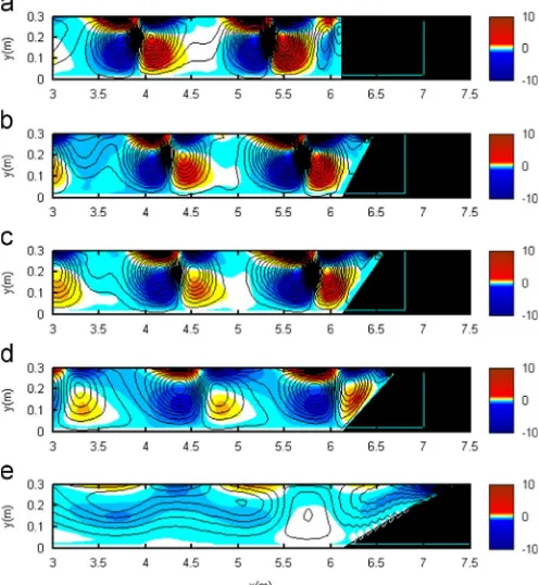
The steady streaming system is the key mechanism in the development of scour/deposition at the bottom. Analysis of this system is highly necessary to understand the source of the differences of scour/deposition patterns as observed above. Then, to further study the effect of breakwater steepness on this system, the steady streaming patterns in front of the five breakwaters were simulated and analyzed.Fig. 12 plots the steady streaming patterns generated by the standing waves inFig. 10. Thisfigure provides two information related to the steady streaming system,
Fig. 11.Bed profile (after 10 T) in front of thefive breakwater cases: (a) vertical
breakwater, (b) 1:1.2-sloped breakwater, (c) 1:1.5-sloped breakwater, (d) 1:2-sloped breakwater, and (e) 1:4-1:2-sloped breakwater.
Fig. 12.Steady streaming system (averaged streamline and horizontal velocity
namely, streamline and distribution of horizontal velocity. The streamline and horizontal velocity were averaged during 10 T after the standing wave developed. The streamline presents the pattern of water particles motion while the magnitude of horizontal velocity can be used to show the direction of water particles movement and the strength of the steady streaming system.
Fig. 12shows that, the re-circulating cells are clearly generated in front of all breakwaters except in the case of 1:4-sloped break-water. It is seen that there are always two primary re-circulating cells rotating in opposite directions at the vicinity of the node. As an example, in the case of vertical breakwater (Fig. 12(a)), at the vicinity of 3.75 m (the location of 2nd node), clockwise and anticlockwise cells are generated at the left and right of the node, respectively. Most likely, these cells are in charge in the develop-ment of deposition ridge at such location (seeFig. 11(a)). The same thing also occurs at the vicinity of 5.4 m (the location of 1st node). Another secondary clockwise cell with smaller size is generated right in front of the breakwater, under the halfway of the 1st antinode and 1st node at around 5.75 m. This cell and the antic-lockwise at the right of 1st node are most likely the source mechanisms that induce the substantial scour in front of the vertical breakwater.
Furthermore, the locations of the re-circulating cells are shifted due to different breakwater steepnesses in accordance with the shifted locations of the node and antinode as shown inFig. 10. As the steepness becomes gentler, the cells are shifted closer to the breakwater and together with the fluid flowing down (return flow) from the top of the slope, they change theflow condition near the toe of the breakwater. The wider scour at the toe as observed inFig. 11(b) is likely caused by the combination of the anticlockwise cell near the toe and the returnflow. While inFig. 11
(c), the returnflow plays a bigger role to cause the narrow scour at the toe and the anticlockwise cell contributes more on the development of the deposition ridge near the toe.
Then, the characteristics of re-circulating are changed in terms of their size, shape, and strength due to different breakwater steepnesses. As expected in the case of vertical breakwater, the fully standing wave produces relatively more symmetric re-circulating cells (Fig. 12(a)). Although the two cells in the vicinity of nodes rotate in opposite directions, their size, shape and strength are almost similar to each other. In addition, the gener-ated re-circulating cells have strength that is higher than the other cases. Then, the strength of re-circulating cells are decreased as the breakwater steepness becomes gentler. It explains why the scour depth and deposition height become smaller for the gentler slope breakwaters as presented in point 2 above.
These symmetrical features are also observed in the case of 1:1.2-sloped breakwater. Then, the unsymmetrical and weaker cells start to develop in the cases of gentler slopes (Fig. 12(c) and (d)). Even in the case of very gentle slope breakwater (Fig. 12(e)), the re-circulating cells are not observed at all and the magnitude of horizontal velocity is decreased substantially. It explains why the scour/deposition pattern is not formed in front of the 1:4-sloped breakwater (Fig. 11(e)). A possible explanation is that when the slope becomes gentler, the dissipation of wave energy is increased due to more space that is available for run-up process. Therefore, in many experimental works, in order to eliminate the reflected waves that can disturb the physical processes being studied in the wave flume, the sloping structures are usually placed at the other end of waveflume to dissipate the wave energy.
Analysis of turbulence parameters was performed and the results showed that there is a strong correlation between the dissipation of wave energy and the generation of turbulence on the slope of the breakwater. Simulation of turbulencefield para-meters in each breakwater case is worthwhile to more clearly show the effect of different breakwater steepnesses on the
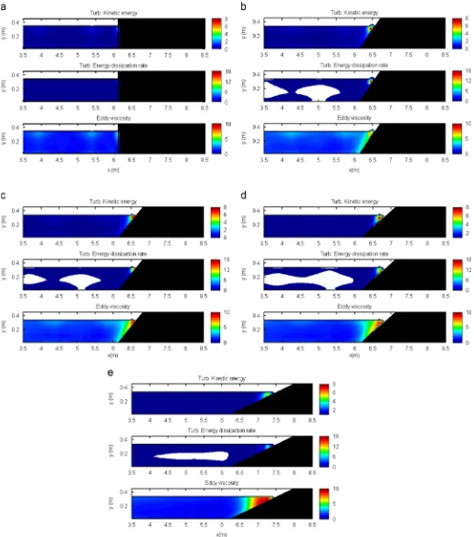
dissipation of wave energy. In the present model, the effects of turbulence were included in the mean flow in terms of eddy viscosity. Thereby, it can be simply assumed that the magnitude of eddy viscosity is representing how much turbulence that is generated in the flow. The distribution of eddy viscosity is an important parameter to assess this feature.Fig. 13provides the distributions of turbulence kinetic energy (k), turbulence energy dissipation rate (ε), and eddy viscosity in front of thefive break-waters. All these parameters were averaged during 10 T.
Fig. 13shows that in all cases,kand εhave almost the same
distribution pattern with different scales of magnitudes and ratios between them. For the vertical breakwater case (Fig. 13(a)), the maximum amount ofkandεcan be observed near the free surface in the interaction zone of wave and breakwater. The same pattern can be observed in the distribution of eddy viscosity, but with different scales of magnitude. However, the generation of turbu-lence in the case of vertical breakwater is the smallest, compared to the other cases. The high level ofk,ε, and eddy viscosity are then observed in the cases of sloped breakwaters, particularly in the wave run-up zone over the slope. The maximum amount ofk andεcan be observed being localized in the farthest tip of the run-up wave for all sloped breakwater cases. While the distribution of eddy viscosity with different scales of magnitude covers a wider area on the slope. It indicates that farther the wave is running up a slope, the turbulent area is increased on the slope. Then, when the wave reaches its maximum run-up distance, the turbulence has been generated in the entire area on the slope that has been passed by the wave. It is important to note that in all sloped breakwater cases, the magnitude of eddy viscosity is distributed restricted only in the area over the slope, and it is not spread to the area in front of the slope. It implies that actually the generated turbulence does not interfere directly the formation of the steady streaming system in front of the sloped breakwaters. However, the dissipation of wave energy accompanied by the generation of turbulence on the slope area is the main source that generates the re-circulating cells with unsymmetrical features and weaker strength as observed inFig. 12(c), (d), and (e). Subsequently, the smaller sizes of scour troughs/deposition ridges (Fig. 11(c) and (d)) and even unchanged bed (Fig. 11(e)) are produced at the bottom. Several important features in the distribution of turbulence field parameters can be observed in Fig. 13. Further analysis of these features is highly important to understand the effects of breakwater steepness on the correlation between the wave energy dissipation and turbulence generation. The order of maximum turbulent kinetic energy,k, and its dissipation rate,ε, in the case of 1:1.2-sloped breakwater (Fig. 13(b)) is the highest while the order of maximum eddy viscosity is the smallest, compared to the other sloped breakwaters. As the slope becomes gentler, the order of maximumkandεare then decreased, while the eddy viscosity is increased. The smallest ofkandε, and the highest eddy viscosity are observed in the case of 1:4-sloped breakwater (Fig. 13(e)).
(gentler slope). This ratio is proportional to the magnitude of eddy viscosity (see Eq.(7)). From all these results it can be concluded that, when the wave run-up over the gentler slope, the wave energy dissipation is increased, in which at the same time the generation of turbulence is also increased, which is particularly presented by the increased eddy viscosity. It also implies that the distribution of
eddy viscosity produced on the slope can be used as the indicator to assess the dissipation of wave energy that occurs in different breakwater steepnesses.
de Best and Bijker (1971) has shown experimentally that for
relatively coarse material, the material is moved in the bed-load mode by the bed shear from the antinode towards the node. Their
Fig. 13.Distribution of turbulencefield parameters (averaged during 10 T) in front of thefive breakwater cases: (a) vertical breakwater, (b) 1:1.2-sloped breakwater,
calculation results showed that the total driving force towards the node is always greater than towards the antinode, so that the net motion of bed-load towards the node can be expected (seede Best and Bijker, 1971for the details). An analysis of sediment transport rate is also presented to understand the mechanism of sediment movement in the five breakwaters. Fig. 14 shows the spatial distribution of total-load sediment transport rate (ST), its gradient, bed profile (as inFig. 11) after 10 T for thefive breakwater cases. The predicted total-load transport rate and its gradient are also time-averaged quantities for 10 T. It is also presented in thefigure the locations of 1st node and 2nd antinode of standing wave, which are according toFigs. 10 and 11. It can be seen in all cases (except the 1:4-sloped breakwater case), the spatial distribution of ST-values is in terms of alternating positive and negative peaks, in which the peaks always occur around halfway between node and antinode. It means that large amounts of sediment transport occur at the halfway. As shown in Eq. (4), the model of bed profile change uses the gradient ofSTto calculate the bed level in a certain location. Thereby, the gradient ofSTcan be used as an indicator that shows the bed elevation. It is interesting to observe inFig. 14
that the scour is related to a positive gradient of the ST, the deposition with the negative gradient, and zero gradient repre-sents no scour and no deposition or zero elevation.
By relating the spatial distribution of ST, its gradient and the locations of scour troughs and deposition ridges, the direction of sediment movement can be simply determined, which is represented by the black arrows in thefigure. As an example,firstly, lets focus the
attention to the location of the node (5.75 m) in the vertical break-water case (Fig. 14(a)). TheST-value in this location is zero, indicating that the sediment at this location is not transported anywhere. However, the gradient ofSTis not zero yet negative, indicating that there is a deposition formed at this location. The node is surrounded by two peaks ofST-values, a negative peak at its right and a positive peak at its left, in which the two peaks are located at the halfway of node and antinode. It indicates that the sediments at the surrounding halfway towards the node, which are eventually deposited at the node. Now, let see in the 2nd antinode location (4.5 m). At this location, zero values ofSTand its gradient are observed. It indicates that in this position the sediments are not moving anywhere and the bed elevation is not changed. Meanwhile, in contrast to the node, the antinode is surrounded by a positive peak at its right (or positive peak at the left of the node) and a negative peak at its left, which are also located at the halfway. It shows that the sediments at the surrounding halfway move away from the antinode. All these results are consistent with the calculation of total driving force conducted byde Best and Bijker (1971).
The same analysis can be performed in the other breakwater cases to understand the development of scour/deposition pattern from the sediment transport rate aspect. The effects of breakwater steepness on the total-load sediment transport rate (ST) can be observed presented inFig. 14. In general, the value ofSTis decreased as the breakwater steepness gettingflatter, even in the case of 1:4-sloped breakwater the transport rate is very small and almost zero. In addition, significant phase changes in the total-load graphics are also observed due to
Fig. 14.Total-load sediment transport rate (ST), gradient ofST, and bed profile (as inFig. 10) after 10 T; (a) vertical breakwater, (b) 1:1.2-sloped breakwater, (c) 1:1.5-sloped
different breakwater steepnesses, which is in tune to the formation of scour troughs and deposition ridges that occur at different locations in each case.
5. Conclusions
A two-dimensional numerical model was developed and applied to study the effects of breakwater steepness on the hydrodynamics of standing wave and scour/deposition pattern in front of five breakwaters with different steepnesses. The model was based on a combination of the RANS equations, VOF method, and ak–εturbulence closure model, which was combined with an empirical sediment transport model ofBailard (1981). The addi-tional terms of bottom shear stress were incorporated into the momentum equations as used byKarambas (1998). Model perfor-mance in predicting the near bottom velocity was evaluated by comparing the numerical results with the experimental data of
Xie (1981) and Zhang et al. (2001) and analytical solution for
standing wave. A very good agreement was observed between the numerical results, analytical solutions and experimental results. In simulating the scour/deposition pattern, the model was validated qualitatively against the experimental data ofSumer et al. (2005)
and the previous numerical results ofGislason et al. (2009a,b)and
Tahersima et al. (2011). The simulated scours/deposition pattern was highly consistent with the experimental data and shows better results than the existing numerical studies. This study has led to a better understanding regarding the correlations between the characteristics of standing waves on the surface, steady streaming systems under the surface, and scour/deposition pattern at the bottom under the effects of different breakwater steep-nesses. In addition, analysis of turbulence field and sediment transport rate was also performed. Based on the present numerical results, some important information can be taken and presented as follows:
In the present model, the additional terms of bottom shear stress in the momentum equations are necessary to produce physical scour/deposition pattern. Without these terms the present model produced an unphysical scour/deposition pattern. Different breakwater steepnesses change interaction of the incident and reflected waves in front of the breakwater. The main mechanism for these changes is the dissipation of wave energy as the wave run-up over the slope of the breakwater. The gentler slope dissipates more energy carried by the incident wave. The gentler breakwater steepness shifts the locations of nodes and antinodes of standing wave closer to the breakwater and reduces the symmetrical feature and the amplitude of standing wave. The steady streaming system becomes more unsymmetrical and weaker for the breakwater with gentler slope. The scour/deposition patterns at the bottom are formed differ-ently due to different breakwater steepnesses. In general, as the slopes become gentler, the magnitudes of scour depth and deposition ridge are decreased, and their locations are shifted closer to the breakwater's toe. For the sloped breakwaters, the generation of turbulence in the flow is restricted only on the wave run-up area. The generated turbulence is not spread into theflow in front of the break-water and does not interfere the steady streaming system. The time-averaged turbulencefield parameters can be used to assess the wave energy dissipation in the sloped breakwater case. When the wave energy is dissipated during the interac-tion of wave and the slope of the breakwater, at the same timethe turbulence is generated on the slope. The gentler produces more turbulence on the wave run-up area.
The mechanism of sediment transport (coarse material) in the case of sloped breakwaters is similar to the vertical breakwater case, which are the sediments moving away from the antinode towards the node. As the breakwater steepness is decreased, the magnitude of the total transport rate is also decreased; the maximum and minimum peaks in the spatial distribution of transport rate are shifted towards the breakwater. Since the decreasing of breakwater steepness weakens the strength of the steady streaming system, there is almost no sediment transported in the case of 1:4-sloped breakwater.Numerical simulations presented in this paper provide insight into the ability of the present model to simulate the detailed hydrodynamics of standing wave and scour/deposition pattern in the front of impermeable breakwaters with different steepnesses. Like previous studies, the numerical results for the bed profile are in need of improvement, and remain a challenge for future studies. Simulation of interaction mechanism offluid and sediment at the bottom can be improved using the two-way coupling method to include the interaction forces betweenfluid and sediment. These interaction forces can only be simulated using more comprehen-sive two-phase models. Although the present model could produce the scour/deposition patterns that consistent with the experimental result and better than the existing models, it must be noted that all the simulated scour/deposition patterns are not in the equilibrium state. As faced in other studies, the computa-tional expense of the RANS-based models has been the main limitation for simulating the equilibrium scour/deposition pattern, which is usually reached for a very long duration. It makes the quantitative comparison using the same time scale with the existing works is still not possible. Numerical methods used in the present model require improvements to improve the running time of the model to be more applicable for practical uses.
Acknowledgments
The author would like to thank the Ministry of Higher Education, Malaysia (MoHE) for financially supporting this study through research grant of Tabung Amanah MLNG-INOS (TE 67901).
References
Bagnold, R.A., 1946. Motion of waves in shallow water: interaction between waves and sand bottom. Proc. R. Soc. Lond. Ser. A 187, 1–15.
Bailard, J.A., 1981. An energetics total sediment transport model for a plane sloping beach. J. Geophys. Res.C11, 10938–10954.
Bakhtyar, R., Barry, D.A., Yeganeh-Bakhtiary, A., Ghaheri, A., 2009. Numerical simulation of surf-swash zone motions and turbulentflow. Adv. Water Resour. 32, 250–263.
Bijker, E.W., 1971. Longshore transport computation. J. Waterw. Harbors Coast. Eng. Div. ASCE 97 (WW4), 687–701.
de Best, A., Bijker, E.W., 1971. Scouring of a sand bed in front of a vertical breakwater (Communications on Hydraulics, Report no. 71-1). Department of Civil Engineering, Delft University of Technology.
Engelund, F.A., FredsØe, J., 1976. A sediment transport model for straight alluvial channels. Nord. Hydrol. 7 (5), 293–306.
FredsØe, J., Deigaard, R., 1992. Mechanics of Coastal Sediment Transport. World Scientific, Singapore.
Gislason, K., FredsØe, J., Sumer, B.M., 2009a. Flow under standing wave, Part1. Shear stress distribution, energyflux and steady streaming. Coast. Eng. 56, 341–362. Gislason, K., FredsØe, J., Sumer, B.M., 2009b. Flow under standing wave, Part2.
Scour and deposition in front of breakwaters. Coast. Eng. 56, 363–370. Hajivalie, F., Yeganeh-Bakhtiary, A., 2009. Numerical study of breakwater steepness
effect on the hydrodynamics of standing wave and steady streaming. J. Coast. Res. SI 56, 658–662.
Hirt, C.W., Nichols, B.D., 1981. Volume offluid (VOF) method for the dynamics of free surface boundaries. J. Comput. Phys. 39, 201–225.
Hughes, S.A., Fowler, J.E., 1991. Wave-induced scour prediction at vertical walls. In: Proceedings of the Conference Coastal Sediments 91, pp. 1886–1899. Irie, I., Nadaoka, K., 1984. Laboratory reproduction of seabed scour in front of
breakwaters. In: Proceedings of the 19th International Conference on Coastal Engineering, Houston, TX, Vol. 2, 26, pp. 1715–1731.
Jonsson, I.G., 1966. Wave boundary layer and friction factors. In: Proceedings of the 10th Coastal Engineering Conference.
Karambas, T.V., 1998. 2DH non-linear dispersive wave modelling and sediment transport in the nearshore zone. In: Proceeding of the International Conference of Coastal Engineering (ICCE), pp. 2940–2953.
Launder, B.E., Spalding, D.B., 1974. The numerical computation of turbulentflow. J. Computational Mech. Appl. Mech. Eng. 3, 269–289.
Lee, K., Mizutani, N., 2008. Experimental study on scour occurring at a vertical impermeable submerged breakwater. Appl. Ocean Res. 30 (2), 92–99. Lin, P., Liu, P.L.F., 1998. A numerical study of breaking waves in the surf zone. J. Fluid
Mech. 359, 239–264.
Nichols, B.D., Hirt, C.W., Hotchkiss, R.S., 1980. SOLA-VOF: a solution algorithm for transientfluidflow with multiple free boundaries (Report LA–8355). Los Alamos Scientific Laboratory, University of Colifornia.
Patankar, S.V., 1980. Numerical Heat Transfer and Fluid Flow. Hemisphere, New York.
Petit, H.A.H., van Gent, M.R.A., van den Boscj, P., 1994. Numerical simulation and validation of plunging breakers using a 2D Navier–Stokes model.
In: Proceedings of the 24th International Coastal Engineering Conference, ASCE, Kobe, Japan, pp. 511–524.
Sumer, B.M., FredsØe, J., 2000. Experimental study of 2D scour and its protection at a rubble-mound breakwater. Coast. Eng. 40, 59–87.
Sumer, B.M., FredsØe, J., 2002. The Mechanics of Scour in the Marine Environment. World Scientific, Singapore p. 552.
Sumer, B.M., FredsØe, J., Lamberti, A., Zanuttigh, B., Dixen, M., Gislason, K., Penta, A.F.D., 2005. Local scour at roundhead and along the trunk of low crested structures. Coast. Eng. 52 (10–11), 995–1025.
Tahersima, M., Yeganeh-Bakhtiary, A., Hajivalie, F., 2011. Scour pattern in front of vertical breakwater with overtopping. J. Coast. Res. SI 64, 598–602.
Torrey, M.D., Cloutman, L.D., Mjolness, R.C., Hirt, C.W., 1985. NASA-VOF2D: a computer program for incompressibleflows with free surfaces (Report LA– 10612-MS). Los Alamos Scientific Laboratory, University of Colifornia.
Whitehouse, R., 1998. Scour at Marine Structures. Thomas Telford Publications, London.
Xie, S.L., 1981. Scouring pattern in front of vertical breakwaters and their influence on the stability of the foundation of the breakwaters (Report). Department of Civil Engineering, Delft University of Technology, Delft, Netherlands.
Yeganeh-Bakhtiary, A., Hajivalie, F., Hashemi-Javan, A., 2010. Steady streaming and
flow turbulence in front of vertical breakwater with overtopping. Appl. Ocean Res. 32, 91–102.