Angular Momentum of a Rotating Dipole.

(1)

ISSN: 2180 - 1843 Vol. 6 No. 1 January - June 2014

Angular Momentum of a Rotating Dipole

17

Angular Momentum of a Rotating Dipole

Mohd Riduan Ahmad

1,2

and Mona Riza Mohd Esa

1,3 1_{Department of Engineering Sciences, Uppsala University, Sweden}

2_{Faculty of Electronic and Computer Engineering, Universiti Teknikal Malaysia Melaka, Malaysia} 3

Faculty of Electrical Engineering, Universiti Teknologi Malaysia, Malaysia riduan.ahmad@angstrom.uu.se

Abstract_{—In this paper, we derive the far field electromagnetic} fields of a rotating half-wave dipole antenna. Theoretically, we have demonstrated that the far electromagnetic fields of a rotating half-wave dipole carry angular momentum in the term of ϕ-ϕ′, which is absent from the stationary half-wave dipole antenna. The term sin(kr−ωt+[ϕ−ϕ']) tells us that the electromagnetic wave propagates outward with the speed of light c_{(evidence from}k₌ω_/c_{) from the dipole along the}r_{axis and} both electric and magnetic fields are spinning (oscillate with ω rad/s) and orbiting (rotating with ω0rad/s) along the raxis with the speed of light. The orbital frequency is evidence from the term _ϕ₋_ϕ'=ω0t−ω0t'=ω0r/c.

Index Terms—angular momentum, electric field, magnetic field, rotating dipole.

I. INTRODUCTION

An electromagnetic system radiates not only energy (linear momentum) but also angular momentum into the far zone as evidence from electrodynamics literature [1,2,3].In this paper, we are motivated to derive the far field electromagnetic fields of a rotating half-wave dipole antenna, in order to demonstrate theoretically that such antenna would radiate angular momentum into the far zone.

II. CURRENT DISTRIBUTION

A thin rod with length L, perfectly conducting, half-wave dipole antenna is located in the x1′x2′plane and are fed at the

midpoint of the rod (x₀₌₀_{) so that the Fourier amplitude of} the current distribution can be written as such

j_ω(x1')=δ(x2')δ(x3')I0cos(ωx1'ν) ˆx1' (1)

where νis the velocity of the current propagation along the rod that is equivalent to the drift velocity of the moving charges. The rod is rotating at an angular frequency ω0around

a fixed axis (ω≠ω0), which is always perpendicular to the rod

and passes through its midpoint.

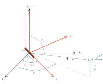
As shown in Figure 1, we introduce a coordinate system (x1,

x2,x3) to describe the fixed observer (the field point) and (x1′,

x2′,x3′) system to describe the source, i.e., a coordinate system

that is fixed in the rod and, consequently, rotates around the

x3′axis (in fact, x3′=x3) with a constant angular frequency ω0.

The direction of the current source in coordinate system (x1,

x2,x3) can be written as such

ˆ

x1'=cos(ϕ') ˆx1+sin(ϕ') ˆx2=Re ( ˆx1+ixˆ2)e−

iω0t'

[image:1.468.252.424.166.306.2]

{

}

(2)

Figure 1: Geometry relevant to the current distribution formulation

where ϕ′ = ω0t′ is the azimuth angle of the source

coordinate system and t′is the retarded time.

Consequently, the Fourier amplitude of the current distribution due to propagating current with angular frequency ωand speed νin the rotating rod with angular frequency ω0

can be re-written as such

j_ω(x1')=I0cos(ωx1'ν)e

−iϕ'

[ ˆx1+ixˆ2]. (3)

III. THE MAGNETIC FIELD

The fields at large distances from the dipole are given in [1]. From these equations we see that

E_ω=c2_B

ω× k

ω (4)

where c is the speed of light and kis the wave vector. Therefore it is sufficient to calculate

B_ω(x)= −i k

4πε0c 2

eikx−x0

x−x0 dx1'

−λ4

λ4

∫

(j_ωeik•(x'−x0)×_k₎ (5) where |x – x0| (or r) is the magnitude of the difference

between position vector x at observation point and the midpoint vector x0at the source coordinate system. Further,

(2)

ISSN: 2180 - 1843 Vol. 6 No. 1 January - June 2014 Journal of Telecommunication, Electronic and Computer Engineering

18

B_ω(x)= −i k 4πε0c

2 ei(kr−ϕ' )

r

dx1'

−λ4

λ4

∫

I0cos ωx1'

ν 

     eik•x1'[( ˆx1+ixˆ2)×k] 

 

  

(6)

The directions of the components of the magnetic field are given by term[( ˆx₁+ixˆ₂)×k]. For transformation to spherical coordinates,

ˆ

x1=sinθcosϕrˆ+cosθcosϕθ −ˆ sinϕϕ ˆ

ˆ

x2=sinθsinϕrˆ+cosθsinϕθ +ˆ cosϕϕ ˆ

Hence,

ˆ

x₁+ixˆ₂=sin

θ

(cos

ϕ

+isin

ϕ

) ˆr+cos

θ

(cos

ϕ

+isin

ϕ

) ˆ

θ

+ (icos

ϕ

−sin

ϕ

) ˆ

ϕ

=eiϕ_(sin

θ

_r_ˆ+_cos

θ

ˆ₊_i

ϕ

_ˆ₎

Therefore, the directions of the components of the magnetic field are

( ˆx1+ixˆ2)×k=ke iϕ

(i

θ

ˆ−cos

θ

ϕ

ˆ) (7)

under paraxial approximation when the wave vector k=(

ω

c)(rr)is propagating in the same direction as radial vector r with the speed of light c. Equation (6) can be re-written as such

B_ω(x)= −iI0 k2

4πε0c 2

ei(kr+ϕ −ϕ' ) r [i

ˆ θ −cosθϕ ˆ]

cosωx1' ν 

     eik•x1'dx1'

−λ4

λ4

∫

(8)

The phase error term

e

ik•x1'_{is very significant due to the}

fact that the length of the dipole L = λ/2 and can be estimated as such

k⋅x₁'=k⋅(x₁+x₂)=kx₁sin

θ

cos

ϕ

+kx₂sin

θ

sin

ϕ

.

Consequently

B_ω(x)= −iI0 k2

4πε0c 2

ei(kr+ϕ−ϕ' ) r [i

cosωx1

ν 

     eik1x1dx1+cos

ωx2

ν 

     eik2x2dx2

  

  

−λ4 λ4

∫

(9)

wherek1=ksin

θ

cos

ϕ

and k2=ksin

θ

sin

ϕ

. Letting κ

denotes either k1 or k2 and ζ denotes either x1 or x2, the

solution for generic integral is given as

cosωζ ν       eiκζdζ 

 

  

−λ4 λ4

∫

= 2k

k2₋κ2cosκ λ

4 

     (10)

when conditionν=cis satisfied. Equation (12) is re-write such that

B_ω(x)= −iI0 k

2πε0c 2

ei(kr+ϕ −ϕ' ) r [i

1 1−(sinθcosϕ)2cos

π 2sinθcosϕ 

     + 1

1−(sinθsinϕ)2cos

π 2sinθsinϕ 

     

    



    

(11)

Transforming this Fourier component back to time domain and taking the (physically acceptable) real part, we obtain, in spherical coordinates

B(t,x)=Re

{

B_ω(x)e−iωt

}

=Re

I0 k

2πε0c 2

ei(kr−ωt+ϕ −ϕ' )

r [ ˆθ +icosθϕ ˆ]

π 2sinθcosϕ 

 

   + 1

π 2sinθsinϕ 

     

    



     

   

   



   

   

=Re

I0 k

2πε0c 2

cos(kr−ωt+ϕ −ϕ')+isin(kr−ωt+ϕ −ϕ')

r

[ ˆθ +icosθ_ϕˆ]

π 2sinθcosϕ 

     + 1

π 2sinθsinϕ 

     

    



     

      

      



      

      

Let

ξ= I0k

2πε0c 2

r

π 2sinθcosϕ 

     + 1

π 2sinθsinϕ 

     

    



    

Then

B(t,x)=ξRe cos(

{

[

kr−ωt+ϕ−ϕ')+isin(kr−ωt+ϕ−ϕ')

]

[ ˆθ +icosθ_ϕˆ]

}

=ξRe

cos(kr−ωt+ϕ−ϕ') ˆθ −sin(kr−ωt+ϕ−ϕ')cosθϕ ˆ

(

)

+i

(

sin(kr−ωt+ϕ−ϕ') ˆθ +cos(kr−ωt+ϕ−ϕ')cosθϕ ˆ

)



   

(3)

ISSN: 2180 - 1843 Vol. 6 No. 1 January - June 2014

Angular Momentum of a Rotating Dipole

19

The time-varying magnetic field in the final form takes place as such

B(t,x)=µ0I0ω

2πcr

1

1−(sinθcosϕ)2cos

π 2sinθcosϕ 

 

   +₁₋_(sin1_θ_sin_ϕ₎2cos

π 2sinθsinϕ 

     

    



    

cos(kr−ωt+[ϕ−ϕ']) ˆθ −sin(kr−ωt+[ϕ−ϕ'])cosθϕ ˆ

[

]

(12)

In the presence of perfect conducting ground parallel to the x3′axis, the total magnetic field observed at the ground level is

the superposition of the magnetic field obtained in Equation (12) and its image. The only component survived at ground level is the component in the direction of

ϕ

ˆ

.

Therefore, the total magnetic field is

B(t,x)= −

ϕ µ

ˆ 0I0

ω

π

cr sin(kr−

ω

t+[

ϕ

−

ϕ

'])cos

θ

1

1−(sin

θ

cos

ϕ

)2cos

π

2sin

θ

cos

ϕ



     +

1

1−(sin

θ

sin

ϕ

)2cos

π

2sin

θ

sin

ϕ



    



    



    

(13)

The total magnetic field carries angular momentum as evidence from the azimuth term ϕ-ϕ′.

IV. THE ELECTRIC FIELD

The electric field can be obtained from Equation (4) as such

E_ω(x)=c2

B_ω(x)×k ω = −iI0

k2

2πε₀ω

ei(kr+ϕ−ϕ' )

r [i( ˆθ ×rˆ)−cosθ( ˆϕ ×rˆ)]

π 2sinθcosϕ 

     + 1

π 2sinθsinϕ 

     

    



    

=I0 k2

2πε0ω ei(kr+ϕ−ϕ' )

r [−

ˆ ϕ +icosθθ ˆ]

π 2sinθcosϕ 

     + 1

π 2sinθsinϕ 

     

    



    

(14)

Transforming this Fourier component back to time domain and taking the (physically acceptable) real part, we obtain, in spherical coordinates

E(t,x)=Re

{

E_ω(x)e−iωt

}

=Re

I0 k2

2πε0ω

ei(kr−ωt+ϕ −ϕ' )

r [−ϕ +ˆ icosθ ˆ θ ]

1

1−(sinθcosϕ)2cos π 2sinθcosϕ 

     +

1

1−(sinθsinϕ)2cos π 2sinθsinϕ 

    



    



     

   

   



   

   

=Re

I0k 2

2πε0ωr

cos(kr−ωt+ϕ −ϕ')+

isin(kr−ωt+ϕ −ϕ')[−ϕ +ˆ icosθθ ˆ]

1

1−(sinθcosϕ)2cos π 2sinθcosϕ 

     +

1

1−(sinθsinϕ)2cos π 2sinθsinϕ 

    



    



     

      

      



      

      

Let

χ= I0k

2

2πε0ωr

1

1−(sinθcosϕ)2cos

π 2sinθcosϕ 

     + 1

π 2sinθsinϕ 

     

    



    

Then

E(t,x)=χRe cos(kr−ωt+ϕ −ϕ')+

isin(kr−ωt+ϕ −ϕ')[−_{ϕ +}ˆ icosθθ ˆ] 

 

  

=χRe

−[sin(kr−ωt+ϕ −ϕ')cosθθ +ˆ cos(kr−ωt+ϕ −ϕ') ˆϕ ]+

i[cos(kr−ωt+ϕ −ϕ')cosθθ −ˆ

sin(kr−ωt+ϕ −ϕ') ˆϕ ] 

  

  



  

(4)

ISSN: 2180 - 1843 Vol. 6 No. 1 January - June 2014 Journal of Telecommunication, Electronic and Computer Engineering

20

The electric field in the final form takes place as such

E(t,x)= − I0k

2πε0cr

π 2sinθcosϕ 

    

+ 1

π 2sinθsinϕ 

     

    



    

sin(kr−ωt+[ϕ−ϕ'])cosθθ +ˆ cos(kr−ωt+[ϕ−ϕ']) ˆϕ 

  

   

(15)

In the presence of perfect conducting ground parallel to the x3′axis, the total electric field observed at the ground level is

the superposition of the electric field obtained in Equation (15) and its image. The only component survived at ground level is the component in the direction of

θ

ˆ

.

Therefore, the total electric field is

   

 

   

 

   

  −

+    

  −

− + − −

=

ϕ θ π ϕ θ

θ ϕ ϕ ω πε

θ

sin sin 2 cos ) sin (sin 1

1

cos sin 2 cos ) cos (sin 1

1

cos ]) ' [ sin( ˆ ) , (

2 2 0

0 _kr _t

cr k I t x E

The total electric field carries angular momentum as evidence from the azimuth term ϕ-ϕ′.

V. CONCLUSION

Theoretically, we have demonstrated that the far electromagnetic fields of a rotating half-wave dipole carry angular momentum in the term of ϕ-ϕ′, which is absent from the stationary half-wave dipole antenna. The term

sin(kr−

ω

t+[

ϕ

−

ϕ

']) tells us that the electromagnetic wave propagates outward with the speed of light c(evidence from k

=ω/c) from the dipole along the raxis and both electric and magnetic fields are spinning (oscillate with ω rad/s) and orbiting (rotating with ω0rad/s) along the raxis. The orbital

frequency is evidence from term

ϕ−ϕ'=ω0t−[ω0t−ω0r/c]=ω0r/c.

REFERENCES

[1] B. Thide ́, Electromagnetic Field Theory (Dover Publications, Inc., Mineola, NY, USA, 2nd edn., in press), URL http://www.plasma.uu.se/CED/Book. ISBN: 978-0-486-4773-2.

[2] F. Tamburini et al., Encoding many channels on the same frequency through radio vorticity: first experimental test New J. Phys. 14, 033001 (2012).