Robustness analysis of covariance matrix

(1)

ROBUSTNESS ANALYSIS OF COVARIANCE MATRIX ESTIMATES

M. Mahot

123

_{, P. Forster}

3

_{, J. P. Ovarlez}

12

_{and F. Pascal}

1

_,

1_{SONDRA, Supelec}

3 rue Joliot-Curie

91190 Gif-sur-Yvette, France phone: + 33 1 6985 1817, melanie.mahot@supelec.fr

2_{ONERA, DEMR/TSI}

Chemin de la Huni`ere,

91761 Palaiseau Cedex, France

3_{SATIE, ENS Cachan, CNRS, UniverSud}

61, Av. du Pdt Wilson, F-94230 Cachan, France

ABSTRACT

Standard covariance matrix estimation procedures can be very affected by either the presence of outliers in the data or some mismatch in their statistical model. In the Spherically Invariant Random Vectors (SIRV) framework, this paper proposes the statistical analysis of the Normalized Sample Covariance Matrix (NSCM) and the Fixed Point (FP) estimates in disturbances context. The main contribution of this paper is to theoretically derive the bias of the NSCM and the FP arising from disturbances in the data used to build these estimates. The superiority of these two estimates is then highlighted in Gaussian or SIRV noise corrupted by strong deterministic disturbances. This robustness can be helpful for applications such as adaptive radar detection or sources localization methods.

1. INTRODUCTION

Many signal processing applications require the estimation of the data covariance matrix. This is the case for instance for source localization techniques such as conventional beamforming and high resolution methods (CAPON, MUSIC, ESPRIT,...) [1, 2, 3]. Adaptive radar and sonar detection methods also depend on the noise covariance ma-trix estimate [4]. In these cases, the estimation accuracy has a strong influence on the resulting performance. However, standard estimation process can be very affected by either the presence of outliers in the data or some mismatch on their statistical model.

In the conventional Gaussian framework, the well-known Sample Covariance Matrix (SCM) [5] is the Maximum Likelihood Estimate (MLE) and is therefore widely used for its good statistical properties : unbiasedness, efficiency, asymptotic Gaussianity,... Unfortunately, this estimate may perform poorly when the noise is not Gaussian anymore. One of the most general and elegant non-Gaussian noise model is provided by the so-called Spherically Invariant Random Vectors (SIRV). Indeed, these models encompass a large number of non-Gaussian distributions, including the Gaussian one. Within this modeling, it has been shown that the Normalized Sample Covariance Matrix (NSCM) and the Fixed Point (FP) are appropriate in terms of statistical performance [6, 7]. Moreover we will show in this paper that the NSCM and FP are also less sensitive to disturbances (outliers) than the SCM.

The authors would like to thank the Direction G´en´erale de l’Armement (DGA) to fund this project.

More precisely, one of the contributions of this paper is to derive the theoretical bias of the NSCM and the FP arising from disturbances. The paper is organized as follows : section 2 formulates the problem while section 3 provides the main results. In section 4, simulations validate the theoretical analysis and illustrate the robustness of these estimates. Finally, section 5 concludes this work.

2. PROBLEM STATEMENT

A SIRV is a non-homogeneous Gaussian process with ran-dom power. More precisely, a SIRV [8] is the product of the square root of a positive random variableτ(texture), and an m-dimensional independent complex Gaussian vectorx

(speckle) with zero mean, covariance matrixM=E(xxH₎

normalized according to Tr(M) =m:

c=√τx. (1)

Nowadays, SIRVs are increasingly used to model impulsive noise. In most applications, the speckle covariance matrix is of great importance (e.g adaptative detection in radar/sonar) and must be estimated if unknown. For that purpose, N independent snapshots y1, ...,yN are usually available.

Ideally, theseNdata should share the same distribution asc

in (1).

However, in many situations, it may happen that some of these data, let us say the K first y1, ...,yK, are outliers

with a different distribution thanc. Thus,y1, ...,yN may be

split into two sets :

yk=pk for 1≤k≤K;

yn=cn=√τnxn forK<n≤N; (2)

wherecn,τnandxnshare the same distribution asc,τandx.

In this paper, the outlierspk will be assumed to be

ran-dom vectors with arbitrary distributions, and our purpose is to study the robustness of two speckle covariance matrix es-timates : the NSCM and the FP. The NSCM, originally intro-duced in [9, 10], is defined by :

c MNSCM=

m N

N

∑

n=1

ynyHn

kynk2

. (3)

Its statistical properties have been derived in [6] in an ideal outlier-free context : (3) is a biased estimate of M,

(2)

unlessMis the identity matrix.

The FP estimate [11, 12, 13], defined as the unique solution of the following equation

c

is obtained in practice, by an appropriate convergent algorithm [11]. It exhibits good statistical performance (consistency, unbiasedness and asymptotic gaussianity) [6] in the outlier-free case.

3. MAIN RESULTS

LetMcdenote a speckle covariance matrix estimate (NSCM, FP, ...). The goal of this section is to derive its robustness to outliers within the framework (2). For that purpose, the additionnal bias∆due to the presence of outliers is defined as

∆=E(cM_|Koutliers)−E(cM_|no outlier). (5)

In the sequel, we will simply writeE(cM)forE(cM_|K out-liers). Two results will be provided for each estimate : a general expression of∆, and a more specific one valid only for a particular type of outliers :

pk=mk+ck, (6)

wherem_kis deterministic and much stronger than the SIRV component : k m_k _k>>kc_k _k. Expression (6) accounts for the so-called ”data contamination” case, often met in some adaptative detection problems. In the sequel, it will be referred to as the ”data contamination model” for outliers.

Theorem 3.1

Let us denoteMNSCM=E(cMNSCM|no outliers). The addi-tional bias (5) due to outliers is given by :

∆_NSCM=−K_NMNSCM+

For the data contamination model (6), the termE

_p

Whenkmkk →∞(very strong data contamination),∆NSCM simplifies to :

∆NSCM=− See Appendix A.

Now let us turn to the FP estimate.

Theorem 3.2

ForN>>K, the additionnal bias (6) due to outliers is given by

In the data contamination model (6), the term

E See Appendix B.

Expressions (7) and (10) show that both the NSCM and the FP are robust estimates since their additional biases do not depend on the outliers norm but solely on the quantities

pk

kpkk

.

This is in contrast with the widely used SCM which is already known to be a poor estimate in impulsive noise. Fur-thermore, when outliers are present and in a SIRV context, the resulting bias is trivially shown to be equal to

∆SCM=

which is obviously very sensitive to strong outliers.

4. SIMULATIONS

(3)

−10 0 10 20 30 40 50 −40

−20 0 20 40 60 80

Power contamination, 20log(σ_α)

Frobenius Norm of delta, 20log(||

∆

||F

) Simulated SCM

Simulated NSCM Simulated FP Theoretical SCM Theoretical NSCM Theoretical FP

Figure 1: Frobenius norm of∆for the SCM, NSCM and FP versus disturbances power for a Gaussian noise.

−10 0 10 20 30 40 50 −40

−20 0 20 40 60 80

Power contamination, 20log(σ_α)

∆

||F

) Simulated SCM

Simulated NSCM Simulated FP Theoretical SCM Theoretical NSCM Theoretical FP

Figure 2: Frobenius norm of∆for the SCM, NSCM and FP versus disturbances power for a K-distributed noise.

In figures 1 and 2 we study the validity of the general expressions (7) and (10), for a single distubance of the form

p=αdwhereα is a random Gaussian variableN ₍₀_,σ_α2₎

and d a fixed unit norm steering vector. Plots give the Frobenius normk.kF(in dB) of∆SCM,∆NSCMand∆FPas

a function of 20log(σ_α). Figure 1 addresses the Gaussian noise case (τn=1 in equation (2)), while in figure 2 the noise is K-distributed (τn follows a Gamma distribution). The K-distribution parameterνis equal to 0.1 which results in a highly impulsive noise.

These simulations prove the validity of the general

expres-−10 −5 0 5 10 15 20

−60 −50 −40 −30 −20 −10 0 10

Power contamination, 10log(||m₁||2)

∆

||F

)

Simulated SCM Simulated NSCM Simulated FP

Approximate expression: SCM Approximate expression: NSCM Approximate expression: FP

Figure 3: Frobenius norm of∆for the SCM, NSCM and FP versus disturbances power for a Gaussian noise: data con-tamination model.

−10 −5 0 5 10 15 20

−60 −50 −40 −30 −20 −10 0 10

Power contamination, 10log(||m 1||

2₎

∆

||F

)

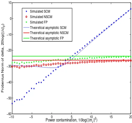
Simulated SCM Simulated NSCM Simulated FP Theoretical asymptotic SCM Theoretical asymptotic NSCM Theoretical asymptotic FP

Figure 4: Frobenius norm of ∆ for the SCM, NSCM and FP versus disturbances power for a K-distributed noise: data contamination model.

sions (7) and (10) of the bias. Furthermore, they show the insensitivity of the NSCM and the FP with respect to the outliers strength, while the SCM’s performance is strongly degraded when the outliers power increases.

(4)

K-distribution. As expected, for largekm1k, experimental

results are close to the approximate expressions. Indeed, theoretical results have been derived under the assumption thatkm1k>>kc1k(cf Remarks 1 and 2).

On the other hand, in figure 3, for low disturbance power, the NSCM and the FP are slightly better than the SCM. However, in figure 4 it is not the case. We also notice a better overall adequacy between experimental and approximate curves for the FP and for the NSCM estimates. We can roughly explain that behavior in the case of highly impulsive noise. Indeed, in this context, one has km1k >> kc1k

with high probability, even for weak disturbances. Thus the approximate expressions remain valid in a wider domain for

km₁_kthan in the Gaussian case.

5. CONCLUSION

In this paper we have investigated the robustness of two covariance matrix estimates, the NSCM and the FP, when part of the data are outliers. In this context, we have derived theoretical formulas of the bias for an arbitrary distribution of the disturbances. In the data contamination case which is met in some applications, we have established simple approximate bias expressions.

These theoretical investigations have been validated by simulations results, and they demonstrate the superiority of the NSCM and the FP over the standard SCM, in terms of robustness. The results are of particular interest in applications such as adaptive radar and source localization methods.

A. PROOF OF THEOREM 3.1

(7) is trivial, therefore we provide only the proof of theorem

3.1 in the data contamination case. Let us rewriteE

_p

This concludes the proof.

B. PROOF OF THEOREM 3.2

Within the framework (2), the FP estimate (4) can be written

c

mean and covariance matrixI

• qk=M−1/2pk.

Previous equation (16) admits a unique solution such that Tr(R) =b m. WhenNtends to+∞and for fixedK, equation (16) tends to

A=mE

It has been proved in [6] that the unique solution of (17) which satisfies Tr(A) =misA=I.

Consequently, when N tends to +∞, Rb solution of equation (16) tends to I, solution of equation (17). This establishes the consistency ofRb. Thus, for largeN, one has

b

R=I+∆Rwherek∆R_k<<kI_k.

Assuming that∆Ris small enough to ensure the validity of a first-order expansion, (16) can be written

I+∆R=m equation may be neglected leading to :

I+∆R=P+N−K

Now, let us define

• δ=vec(∆R)b ,i=vec(I),tn=

zn

kznk

(5)

• δNSCM=vec(RbNSCM−I) =vec(∆RNSCM),where vec(.)

denotes the operator which reshapes them_×nmatrix el-ements into amncolumn vector.

Then, one obtains

i+δ=p+N−K

N

i+δNSCM+

m N₋K

N

∑

n=K+1

(t∗_n⊗tn)(t∗_n⊗tn)H_δ !

(19)

where∗denotes the conjugate operator and⊗the Kronecker product.

By noticing that Tr(∆R) =0impliesiHδ =0, the pro-jection of equation (19) onto the orthogonal subspace of i

gives :

δ =Π⊥i p+

N₋K

N Π

⊥

i δNSCM+

_m

NΠ

⊥ i

N

∑

n=K+1

(t∗_n_⊗tn)(t_n∗_⊗tn)HΠ⊥i δ !

,

whereΠ⊥i =I−

1 mii

H

and where the equalityΠ⊥i δ =δ has

been used.

This is equivalent to

b

αδ=Π⊥i p+

N₋K

N Π

⊥

i δNSCM. (20)

whereαb=I₋ m

NΠ

⊥ i

N

∑

n=K+1

(t∗_n⊗tn)(t∗_n⊗tn)H_Π⊥ i

!

.

It may be shown that

b α P

−−−→

N→∞ α= (I−

1 m+1Π

⊥ i ),

where₋_→P denotes the convergence in probability.

Therefore, αb may be replaced by α in (20) without affecting the asymptotic distribution ofδ. By noticing that

αδ = m

m+1δ,

(20) leads to

δ=m+1

m Π

⊥ i p+

m+1 m

N₋K N δNSCM,

where the identityiH_δ

NSCM=0 has been used.

Using the unvec operator (the vec inverse operator ), one obtains

∆R=m+1

m

P₋Tr(P)

m I

+m+1

m

N₋K

N ∆RNSCM.

Since ∆FP = E[cMFP −M] = E[M1/2∆RM1/2] and

E[RbNSCM] =I, the previous equation leads to theorem 3.2 which concludes the proof.

Starting from this general result, the additive bias obtained in the data contamination model can easily be calculated, using a similar method as in the NSCM case.

REFERENCES

[1] J. Capon, “High-resolution frequency-wavenumber spectrum analysis,” Proc. IEEE, vol. 57, no. 8, pp. 1408–1418, August 1969.

[2] R. O. Schmidt, “Multiple emitter location and signal parameter estimation,”IEEE Trans.-ASSP, vol. 34, no. 3, pp. 276–280, March 1986.

[3] R. Roy and T. Kailath, “ESPRIT-Estimation of signal parameters via rotational invariant techniques,” IEEE Trans.-ASSP, vol. 37, no. 7, pp. 984–995, July 1989. [4] S. M. Kay, Fundamentals of Statistical Signal

Pro-cessing - Detection Theory, vol. 2, Prentice-Hall PTR, 1998.

[5] T. W. Anderson, An Introduction to Multivariate Sta-tistical Analysis, John Wiley & Sons, New York, 1st edition, 1958.

[6] F. Pascal, P. Forster, J.-P. Ovarlez, and P. Larzabal, “Performance analysis of covariance matrix estimates in impulsive noise,”IEEE Trans.-SP, vol. 56, no. 6, pp. 2206–2217, June 2008.

[7] S. Bausson, F. Pascal, P. Forster, J.-P. Ovarlez, and P. Larzabal, “First and second order moments of the normalized sample covariance matrix of spherically in-variant random vectors,” IEEE SP Letters, vol. 14, no. 6, pp. 425–428, June 2007.

[8] K. Yao, “A representation theorem and its applica-tions to spherically invariant random processes,”IEEE Trans.-IT, vol. 19, no. 5, pp. 600–608, September 1973. [9] E. Conte, M. Lops, and G. Ricci, “Adaptive radar de-tection in compound-gaussian clutter,” Proceedings of Eusipco, pp. 526–529, September 1994.

[10] F. Gini, M. V. Greco, and L. Verrazzani, “Detection problem in mixed clutter environment as a gaussian problem by adaptive pre-processing,” Electron. Lett. 31 (14), pp. 1189–1190, July 1995.

[11] F. Pascal, Y. Chitour, J.-P. Ovarlez, P. Forster, and P. Larzabal, “Covariance structure maximum likelihood estimates in compound gaussian noise : Existence and algorithm analysis,”IEEE Trans.-SP, vol. 56, no. 1, pp. 34–48, January 2008.

[12] E. Conte, A. De Maio, and G. Ricci, “Recursive estima-tion of the covariance matrix of a compound-Gaussian process and its application to adaptive CFAR detec-tion,” IEEE Trans.-SP, vol. 50, no. 8, pp. 1908–1915, August 2002.