Fluctuations Mitigation of Variable Speed Wind Turbine through Optimized Centralized Controller

ISSN: 1693-6930

accredited by DGHE (DIKTI), Decree No: 51/Dikti/Kep/2010 703

Fluctuations Mitigation of Variable Speed Wind Turbine

through Optimized Centralized Controller

Ali Mohammadi*, Sajjad Farajianpour, Saeed Tavakoli, and S. Masoud Barakati Faculty of Electrical and Computer Engineering, University of Sistan and Baluchestan, Iran

e-mail: a.mohammadi@mail.usb.ac.ir*, s.farajian@mail.usb.ac.ir, tavakoli@ece.usb.ac.ir, smbaraka@ece.usb.ac.ir

Abstrak

Suatu sistem konversi energi angin (WECS) yang mengandung jenis pembangkitan tenaga angin yang dapat diatur dan terhubung dangan jala jala sangat diperlukan untuk dikendalikan. Dalam tulisan ini setiap komponen model WECS secara sistematik disajikan dan diintegrasikan serta divalidasi. Sifat alamimiah dari WECS yang non linier dan struktur sistem yang kompleks yang diasumsikan sebagai sistem yang memiliki masukan jamak dan keluaran jamak (MIMO), telah membuat sistem ini sulit untuk dibuat strategi kendalinya. Untuk menyederhanakan rancangan kendali, suatu pengendali terpusat yang bersesuaian dengan model sistematik tadi telah diterapkan. Untuk menambah unjuk kerja pengendali terpusat, suatu algoritma generik untu optimasi disertakan. Hasil simulasi menunjukkan efektitifas strategi kendali yang diusulkan untuk mengatasi perpindahan fluktuasi.

Kata kunci: algoritma genetik (GA), masukan jamak dan keluaran jamak (MIMO), migitasi fkuktuasi, pengendali optimum terpusat, sistem konversi energi angina (WECS)

Abstract

A wind energy conversion system (WECS) including a variable wind turbine in grid-connected mode is considered to control. In this paper, each component of WECS model is systematically presented and then the integrated overall model is validated.Regarding to nonlinear nature of WECS and the complex system structure as multiple-input multiple-output (MIMO), it is difficult to find a proper control strategy. To simplify the control design, a centralized controller, which is compatible with systematic modelling, is employed. In addition, to enhance the centralized controller performance, an optimization based on genetic algorithm (GA) is accomplished. Simulation results demonstate the effectivesness of the proposed control startegy to mitigation fluctuations.

Keywords: fluctuations mitigation, genetic algorithm (GA), optimized centralized controller, multiple-input multiple-output (MIMO), wind energy conversion system (WECS)

1. Introduction

Wind energy importance from standpoint of economical, environmental, and accessibility aspects attracts much attention to itself rather than other energy types [1]. In spite of its advantages, it contains operation problems as intermittent capture results in low efficiency, poor naturally controllability and predictability [1]. Hence, wind energy conversion system (WECS) control is undeniably considered as a problem to its operation. Works done in this issue differs from standpoint of control methods, the controlled variables, and the system requirements to meet.

controllers with the capability to dispatch power among generator, grid and the battery . In [6], control design are established with small signal analysis to take account into the damping and stability parameters convertible into multi-objective optimization based on differential evolution (DE) to obtain optimal results. Another method is based on nonlinear robust controller to meet both requirements on the network and considering the characteristics system [7].

In previous works, control strategies are accordance with predefined objective. In this study, an attempt is made to employ a simple and easily-implementing strategy in optimized centralized manner to achieve enhanced properties instead of sophisticated methodologies.

This paper is organized as follows: Each compartment of WECS modelling including drive train, power electronic converter, and the generator dynamically are independently presented and the overall equations are integrated and validated through simulation. In section2.8centralized controller structure applied to WECS is explained and finally with respect to contrlled variables, control design is accomplished using GA. Finally, last section is dedicated to conclusions.

2. Research Method

Generally, to design a realistic controller systematically, it necessitates having the model represented in state space equations. Thus, there has been an attempt to model each component of WECS independently and obtain the overall model in valid manner. Wind turbine is the major component of a WECS to convert wind energy into aerodynamic. The drive train is necessary to translate aerodynamic into mechanical energy. The generator is about to produce electrical power, being WECS heart. There should be a mechanism to smooth the fluctuating power corresponding to different wind speed which is applicable through power conditioner. Representation of these components are organized as follows.

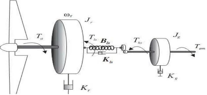
Figure 1. Drive train two-mass model

2.1. Drive Train

Drive train model should be represented so that it considers adequate description and avoids extra computation especially in large power system. The most common models are two-mass and six-two-mass [8]- [10]. Latter includes high order, thus it is not appropriate for large power system. As two-mass model features adequate accuracy and decreasingly computation, it is the best choice to consider. In this model, all masses are lumped at low and high speed shaft. The inertia of the low speed shaft comes mainly from the blades and the inertia of the high speed shaft from the generator (Figure 1). After writing Newton law for low-speed and high-speed shaft and taking into account the self damping of turbine and generator, mutual damping and the system stiffness, state space representation is obtained as follows:

(

t s t t

)

J 1

t T T Dω

ω

t − −

=

   

 

− +

= J1 e s g g

g D ω

n T T

-ω

g

& ₍₂₎

    

  

− +

    

  

− =

n ω ω D n ω ω K

T_{s s t} g _{s t} g

& &

& ₍₃₎

where,ω_t,

g

ω ,T_sangular speed of the turbine and the generator and shaft torque,T_t aerodynamic torque,Te the generator electromagnetic torque,Jt ,Jg turbine and the generator inertia, Dt, Dg self damping of the turbine and the generator, Ks, Ds stiffness and mutual damping and n, the gearbox ratio.

To make modelling more realistic, it is necessary to incorporate aerodynamic torque and electromagnetic torque in the following subsections.

2.2. Aerodynamic Torque

One can model this torque through dividing power captured from the wind by the rotational turbine speed [1] as:

( )

t p 3 w r air t

ω λ β, c v A

ρ

2 1

T = (4)

where, air density, Ar the rotor area swept by the blades, vw effective wind speed met by the rotor and power coefficient, in a variable speed turbine, being a function of the tip speed ratio and pitch angle. Hence, wind speed and pitch angle models are needy to be represented.

2.3. Wind Speed

One model to consider, is presented as superposition of four component including the average value, ramp component, gust component and noise component [11] . With respect to the turbulent described in the frequency domain while the others in time, a conflict encountered during the calculation. Another model which overcomes this problem is composed of two components [12]: low frequency and high frequency. This model is given by sum of mean wind speed and a random process in sinusoidal term as:

) t cos(ω A A

v _{i i}

N

1 i

i 0

w = +

∑

+ϕ

=

(5)

where , A0denotes wind speed mean calculated on a time horizon usually 10 minutes, Ai the amplitude of i-th harmonic in terms of the discrete angular frequency and the corresponding power spectral density obtained by (6) and ϕ_iis generated in a uniform random distribution on interval [−π,π].

(

vv i 1 vv i

)(

i 1 i

)

2 1

i s (ω ) s (ω ).ω ω

π 2

A = ₊ + ₊ − (6)

( )

6 5 2

m m 2

v ωL 1

v L 0.475σ ω

S

   

   

     

+

= . (7)

Considering wind speed passing through the blades, high frequency damping and shadow effect are about to be modelled. High frequency damping can be approximately represented as a low pass filter [15].

1

τs

1 H(s)

+

= (8)

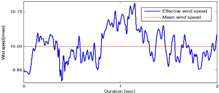
Shadow effect results in periodic torque pulsation caused by passing any blade across the tower. This phenomenon is modelled by adding a sinusoidal periodic torque at N times mechanical speed where N is blades number [16]. Figure 2 demonstartes the wind speed in time domain, considering the effective model above. The Wind tunnel parameteres are available in Appendix I.

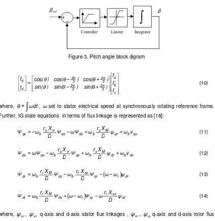
2.4. Pitch Angle Model

To track desired pitch angle, a control system is needed. This task is accomplished via the hydraulic actuator. Pitch angle dynamic is represented as a first-order constrained by the amplitude and derivative of the output pitch (Figure 2). With the assumption to working in linear region, state space to pitch angle is yielded as Equation (9) where β_ref denotes desired pitch angle and τβtime constant. Practically,βranges from −2

o

to 3o and varies at a maximum rate of ±10 o/s [17] .

(

β β

)

τ 1 β _ref

β − =

&

(9)

2.5. Generator Model

To consider the electromagnetic torque meaningfully, it is necessary to develop all dynamics associated to the generator. In this study, squirrel cage induction generator (IG) is employed. Due to simplicity, machine equations are described at dqo reference frame.

Figure 2. Wind speed simulation

Hence, it is essential to transform abc coordinates into synchronously rotating dqo reference frame through Park transformation as follows [18]:

0 1 2

9.85 10.00 10.15

Duration [sec]

W

in

d

s

p

e

e

d

[

m

/s

e

c

]

Figure 3. Pitch angle block digram

                  + − + − =       c b a 3 2π 3 2π 3 2π 3 2π d q f f f ) sin(θ ) sin(θ ) sin( ) cos(θ ) cos(θ ) cos( f f θ θ (10)

where, θ=

∫

ω_dt, ωset to stator electrical speed at synchronously rotating reference frame. Further, IG state equations in terms of flux linkage is represented as [18]:

qs b qr M s b ds qs rr s b

qs ψ ω v

D X r ω ωΨ Ψ D X r ω

Ψ& =− − + + (11)

ds b dr M s b qs rr s b qs

ds ψ ω v

D X r ω Ψ D X r ω ωΨ

Ψ& = − + + (12)

(

r

)

dr

qr ss r b qs M r b

qr Ψ ω ω ψ

D X r ω Ψ D X r ω

Ψ& = − − − (13)

(

)

dr

ss r qr r ds M r b dr ψ D X r ω Ψ ω ω Ψ D X r ω

Ψ& = + − − (14)

where,

ψ

_qs,

ψ

_qs q-axis and d-axis stator flux linkages ,

ψ

_qr,

ψ

_drq-axis and d-axis rotor flux

linkages,X_ss = X_ls+X_M, X_rr =X_lr +X_M, D=X_ssX_rr −X_M2, rs, rr stator and rotor resistances, Xls, Xlr stator and rotor leakage reactances and XM magnetization reactance, ω,ωr ,ω_bstator electrical angular speed, rotor electrical angular speed and base angular speed, v_qs,

ds

v , q-axis and d-axis stator voltages. Finally, the developed electromagnetic torque is computed in terms of the flux linkages and poles number (p) as:

(

qs dr ds qr

)

b M

e Ψ Ψ Ψ Ψ

Dω X 2 p 2 3

T = − (15)

Alternatively, IG currents are calculated in terms of flux linkages in the following matrix.

            Ψ Ψ Ψ Ψ             − − − − =             dr qr ds qs ss M ss M M rr M rr dr qr ds qs X X X X X X X X D i i i i 0 0 0 0 0 0 0 0 1 (16) ref

β

β

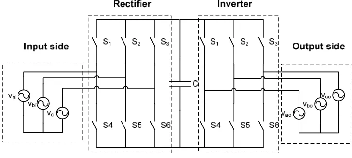
Figure 4. VSC-VSC topology

2.6. Converter Model

A converter plays a prominent role in power conditioning. Among various structures and topologies, back-back VSCc in full-rated scheme is employed (Figure 4) in light of flexibility it features [19]. To finalize modelling, it is adequate to develop vqs and vds through dynamics imposed by the converter. For simplification of control design, the converter model should be accomplished in fundamental frequency neglecting switching dynamics, and in dqo reference frame to be compatible with IG model. Model presented in [20] has above both properties where linear equations with constant frequencies assumption are represented in terms of input and output currents and capacitor voltage as follows:

[

i qi i i di qi qin

]

i

qi R i Lω i v v

L 1

i& = − − + − (16)

[

i qi i i di qi qin

]

i

qi Ri Lωi v v

L 1

i& = − − + − (17)

[

i di i i qi di din

]

i

di R i Lω i v v

L 1

i& = − + + − (18)

[

o qo o o do qo qou

]

o

qo R i L ω i v v

L 1

i& = − − − + (19)

[

o do o o qo do dou

]

o

do R i L ω i v v

L 1

i& = − + − + (20)

[

qin din qou dou

]

d i i i i

4 3 C 1

v& = + − − (21)

where, iqi,, idi are q-axis and d-axis currents coming from input, iqo, idoq-axis and d-axis output currents going to output, vd capacitor voltage, and

)

α

sin(α

i A

i_qin = _{mi qi mi} − _i ,i A i cos(α α )

i mi di

mi

din = − ,iqou =Amoiqosin(αmo −αi),

)

α

cos(α

i A

i_dou = _{mo do mo} − _o ,v 0.5v sin(α α ) i mi d

) α sin(α 0.5v

v_dou = _{d mo}− _o v 0.5v cos(α α ) o mo d

dou = − ,vqi =visin(αi),vdi =vicos(αi ), )

sin(α

v

v_qo= _{o o} , v v cos(α ),

o o

do = vi, voamplitude of the input and output voltage sources, Ri, Li input resistance and inductance, Ro, Lo output resistance and inductance, C, capacitor capacity of dc-link between two converters,ω_i,

o

ω input and output electrical rotational speeds,

i α ,

o α

phase angle of the input and output voltages,Ami, αmi, Amo, αmo amplitude and phase modulation indices of input and output converters. In this model, pulse width modulation (PWM) technique from transforming switching reference frame into dqo is converted to modulation indices as converter inputs. Note that amplitude and phase modulations are definably on interval [0 1] and [-_π, _π], respectively.

2.7. Overall Model of WECS

To achieve the overall modelling, it is essential to integrate the shared-variable equations and eliminate equivalent variables and form the state space representation as follows: ( ) , v ω a Ψ X ω L ω a Ψ D X X r L ω D )X r (R ω a Ψ ω Ψ D ωX L ω a Ψ D X r R ω D X r L ω a Ψ qou b 1,0 dr M r o b 1,0 qr 2 M ss r o 2 b M s o b 1,0 ds ds rr o b 1,0 qs rr s o b 2 M r o 2 b 1,0 qs 2 + +       − + +       + −         ₊ − = D & ( ) , v ω a Ψ D X X r L ω D )X r (R ω a Ψ X ω L ω a Ψ D X r R ω D X r L ω a Ψ ω Ψ D ωX L ω a Ψ dou b 1,0 dr 2 M ss r o 2 b M s o b 1,0 qr M r o b 1,0 ds rr s o b 2 M r o 2 b 1,0 qs ds rr o b 1,0 ds 2 +       − + + −         ₊ − +       + = D &

(

_r

)

_dr, qr ss r b qs M r b

qr Ψ ω ω ψ

D X r ω Ψ D X r ω

Ψ& = − − −

(

_r

)

_qr r ss _dr,

ds M r b dr ψ D X r ω Ψ ω ω Ψ D X r ω

Ψ& = + − −

[

_{i qg i i dg qg qgn}

]

,

i

qg Ri Lωi v v

L 1

i& = − − + −

[

_{i dg i i qg dg dgn}

]

,

i

dg Ri Lωi v v

L 1

i& = − + + −

, )i α sinos(α A a )i α sin(α A a )Ψ α cos(α A D X a )Ψ α sin(α A D X a )Ψ α cos(α A D X a )Ψ α sin(α A D X a v dg i mi mi qg i mi mi dr o mo mo M qr o mo mo M ds o mo mo rr qs oi mo mo rr d − + − + − + − + − − − − = 0 , 7 0 , 7 0 , 7 0 , 7 0 , 7 0 , 7 & , T J 1 T nJ 1 ω J D ω _e g s g r t t

r =− + +

& , T nJ D T J D T J n 1 J 1 ω J D D ω J D D T _e g s t t s s g 2 t r g g s t t t s

s _ + +

      + −         − −       −

= s Ks Ds

n K 1 & . β τ 1 β τ 1 β _ref β β + − = & (22)

where subscript g denotes grid variables replaced for input variable subscript i and

, 1 rr o b 1,0 D X L ω 1 a −       + = . C 0.75 a_7,0 =

To make sure of valid modelling, the simulated WECS is proposed to inject active and

, T J 1 T J 1 ω J D ω _t t s t t t t

t =− − +

reactive power conveniently in an open loop manner.

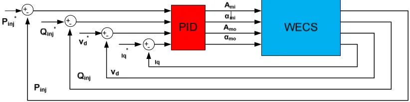
2.8. Control Design

For the MIMO system under study, a centralised controller based on PID in cascaded scheme (Figure 5) is employed, due to its easy implementation and common application in industry. Variables to problem design are injected reactive and active power into the grid, q-axis current and dc-link voltage. Compensator dimension with respect to manipulated and controlled variables is assigned as 4×4. As WECS under study is extremely nonlinear, PID coefficients assignment is a challenging task to meet the best performance. In this study, there has been an attempt to employ the approach including simple implementation using GA rather than methods based on control principle as pole placement. As a PID includes Kp, Pi, Td coefficients, totally, there are 16 optimal parameters. The aim to control is to have the most optimal performance in reference tracking. Among different performance indices common in control principle, Integral Abs Error (IAE) is preferred to others due to involving reasonable view of error reduction. This multi-objective problem is easily convertible into single objective through weighted-sum method [21] as follows:

∑

= = 4

1 i

i iIAE C F(k)

min (23)

where C_i, IAE_i are the weight and IAE asscociated to the ith controlled variable.

3. Results and Analysis

In this section, each component is indepedency simulated and after assurrance of their validation, them all integrated to represent a WECS and then controlled through the proposed optimized strategy. System under syudy is composed of variable wind turbine driven by IG conditioning with Full–rated converter in grid-connected mode. All parameteres regarding to the simulations are given in Appendix I.

Figure 5. Controller configuration

Using Equations (11)-(14), a simulation is started by running IG initially in motoring mode at t=0 sec and then wind turbine applied into generator at t=2 sec. During the starting, all states after a transient behavior, reached steady state values and speed machine was increased till close to synchronous speed (Figure 6). Te also was fixed to zero after meeting a maximum value, presenting natural behavior of IG. After switching in generative mode integrated into wind turbine, machine performed as so to inject power into the grid, being evident from negative final value of Te, which is the sign of machine working generatively.

Figure 6. IG validation simulation

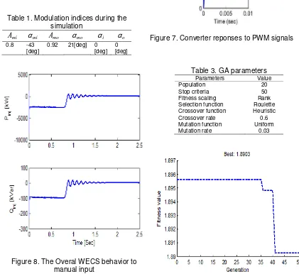
Table 1. Modulation indices during the simulation

mi

A α_mi A_mo α_mo α_i α_o 0.8 -43

[deg]

0.92 21[deg] 0 [deg]

0 [deg]

Figure 7. Converter reponses to PWM signals

Figure 8. The Overal WECS behavior to manual input

Table 3. GA parameters Parameters Value

Population 20

Stop criteria 50 Fitness scaling Rank Selection function Roulette Crossover function Heuristic Crossover rate 0.6 Mutation function Uniform Mutation rate 0.03

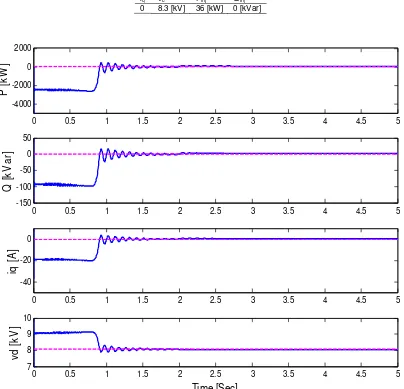
Table 2. Reference values for converter simulation iq* vd* Pinj* Qinj*

0 8.3 [kV] 36 [kW] 0 [kVar]

Figure 10. Controlled variables vs. desired through optimized controller

Furtehrmore, the capacitor has been a reactive interface to help active and reactive power transfer, maintaining its voltage.

Sunsequently, afterward all models were validated, the main task to check the overall model, obtained by equations (22), is accomplished. To operate IG generatively, it is required to work initially as a motor to absorb needy active and reactive power to provide its magnetizing current. At t=2 sec, it is switched into generative mode with input, transiting some damped oscillations, it begins to inject active and reactive power corresponding to control signal applied (Figure 8), hence WECS model is validated.

Centrailised controller optimized via GA is embedded over WECS to track as accurate responses as possible in comparison to desired. Reference values during the simulation are shown in Table II.

GA was performed to solve objective (23) including parameters as tabl III.GA managed to obtain optimal coefficients in 51 generations results in objective (23) to 1.8994 (Figure 9). Simulation results to reponses show successful performance in flutuation mitigation resulted from GA based on PID in error reduction (Figure 10).

0 0.5 1 1.5 2 2.5 3 3.5 4 4.5 5

-4000 -2000 0 2000

P

[

k

W

]

0 0.5 1 1.5 2 2.5 3 3.5 4 4.5 5

-150 -100 -50 0 50

Q

[

k

V

a

r]

0 0.5 1 1.5 2 2.5 3 3.5 4 4.5 5

-40 -20 0

iq

[

A

]

0 0.5 1 1.5 2 2.5 3 3.5 4 4.5 5

7 8 9 10

Time [Sec]

v

d

[

k

V

4. Conclusion

A grid-connected IG-driven WECS equipped with FRC converter is dynamically modelled at fundamental frequency. Centralized controller based on PID due to its dramatic application was embedded over WECS in cascade structure. PID performance was optimally augmented through GA so that, considering multiple controlled variables and multi-objective system was convertible into single-objective via weighted-sum method. Simulation results verified proper performance of the proposed strategy. Future work will contain incorporating a system storage and employing the decentralized controller to power quality problems at variable wind speed and load demands. In addition investigating of system robustness especially in uncertainty condition will be performed.

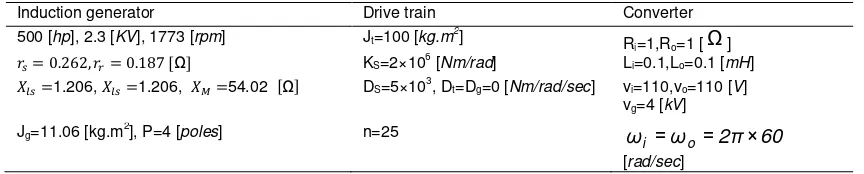
Appendix I

Table 4. WECS parameters during the simulations

References

[1] Mathew S. Wind Energy Fundamentals Resource Analysis and Economics. Springer-Verlag Berlin Heidelberg. 2006.

[2] Haque M. E., Negnevitsky M. and Muttaqi K. M. A Novel Control Strategy for a Variable-Speed Wind Turbine With a Permanent-Magnet Synchronous Generator. IEEE Trans. on Industry Applications. 2010; 46(1).

[3] Hu J., Nian H., Hu B., He Y. and Zhu Z. Q. Direct Active and Reactive Power Regulation of DFIG Using Sliding-Mode Control Approach. IEEE Trans. on Energy Conversion. 2010; 25(4).

[4] Tan K. and Islam S. Optimum Control Strategies in Energy Conversion of PMSG Wind Turbine System Without Mechanical Sensors. IEEE Trans. Energy Conversion. 2004; 19(2).

[5] Abedini A. and Nikkhajoei H. Dynamic Model and Control of a Wind-turbine Generator with Energy Storage. IET Renew. Power Gener. 2011; 5(1): 67–78.

[6] Yang L., Yang G.Y., Xu Z., Dong Z.Y., Wong K.P. and Ma X. Optimal Controller Design of a Doubly-fed Induction Generator Wind Turbine System for Small Signal Stability Enhancement. IET Gener., Transm. & Dist. 2010; 4(5): 579-597.

[7] Hu Ji., Nian H., Hu B., He Y. and Zhu Z.Q. Direct Active and Reactive Power Regulation of DFIG using Sliding-mode Control Approach.IEEE Trans. Energy Convers. 2010; 25(4): 1028-1039. [8] Akhmatov V. Variable-speed Wind Turbines with Doubly-fed Induction Generators. Part I. Modelling

in Dynamic Simulation Tools, Wind Engineering. 2002; 26(2): 85–108.

[9] Ackermann T. Wind Power in Power Systems. John Wiley & Sons, Ltd. Chichester. 2005: 536–546. [10] Papathanassiou S. A. and Papadopoulos M. P. Mechanical Stress in Fixed Speed Wind Turbines

due to Network Disturbance. IEEE Transactions on Energy Conversion. 16(4): 361–363.

[11] Anderson P. M. and Bose A. Stability Simulation of Wind Turbine Systems. Power Apparatus and Systems. 1983; 102(12): 3791-3795.

[12] Nichita C., Luca D., Dakyo B. and Ceanga E. Large Band Simulation of the Wind Speed for Real Time Eind Turbine Simulators. IEEE Trans. on Energy Conversion. 2002; 17(4): 523 – 529.

[13] Burton T., Sharpe D., Jenkins N. and Bossanyi E. Wind Wnergy Handbook. John Wiley & Sons, New-York. 2001.

[14] Munteanu. I., Bratcu A. I., Cutululis N. A, Ceanga E. Optimal Control of Wind Energy Systems: Towards a Global Approach. Advances in Industrial Control. Springer–Verlag London. 2008.

[15] Wu J., Dong P., Yang J.M. and Chen Y.R. A Novel Model of Wind Energy Conversion System. in Proc. DRPT2004. IEEE International Conf. on Electric Utility Deregulation and Power Technologies. April 2000.

[16] Slootweg J.G., Polinder H., and Kling W.L. Representing Wind Turbine Electrical Generating Systems in Fundamental Frequency Simulations. IEEE Trans. on Energy Conversion. 2003; 18(4): 516-524.

[17] Bianchi F. D., Battista H. D. and Mantz R. J. Wind Turbine Control Systems. Advances in Industrial Control.Springer–Verlag London. 2007.

Induction generator Drive train Converter

500 [hp], 2.3 [KV], 1773 [rpm] Jt=100 [kg.m

2

] _R

i=1,Ro=1 [Ω]

ݎ௦= 0.262,ݎ௥= 0.187 [Ω] KS=2×106 [Nm/rad] Li=0.1,Lo=0.1 [mH]

ܺ௟௦=1.206, ܺ௟௦=1.206, ܺெ=54.02 ሾΩሿ DS=5×103, Dt=Dg=0 [Nm/rad/sec] vi=110,vo=110 [V]

vg=4 [kV]

[18] Krause P. C., Wasynczuk O. and Sudhoff S. D. Analysis of Electric Machinery. IEEE Press. 1994. [19] Anaya-Lara O., Jenkins N., Ekanayake J., Cartwright P. and Hughes M. Wind Energy Generation

Modelling and Control. John Wiley & Sons. 2009.

[20] Nikkhajoei, H., Iravani, R. Dynamic Model and Control of AC-DC-AC Voltage-Sourced Converter System for Distributed Resources. IEEE Trans. Power Deliv. 2007: 22(2): 1169–1178.