Time domain noise reduction based on an

Time-domain noise reduction based on an orthogonal

decomposition for desired signal extraction

Jacob Benesty

INRS-EMT, University of Quebec, 800 de la Gauchetiere Ouest, Suite 6900, Montreal, Quebec H5A 1K6, Canada

Jingdong Chen

Northwestern Polytechnical University, 127 Youyi West Road, Xi’an, Shaanxi 710072, China

Yiteng (Arden) Huang

WeVoice, Inc., 1065 Route 22 West, Suite 2E, Bridgewater, New Jersey 08807

Tomas Gaensler

mh acoustics LLC, 25A Summit Avenue, Summit, New Jersey 07901

(Received 22 December 2011; revised 13 April 2012; accepted 16 May 2012)

This paper addresses the problem of noise reduction in the time domain where the clean speech sample at every time instant is estimated by filtering a vector of the noisy speech signal. Such a clean speech estimate consists of both the filtered speech and residual noise (filtered noise) as the noisy vector is the sum of the clean speech and noise vectors. Traditionally, the filtered speech is treated as the desired signal after noise reduction. This paper proposes to decompose the clean speech vector into two orthogonal components: one is correlated and the other is uncorrelated with the current clean speech sample. While the correlated component helps estimate the clean speech, it is shown that the uncorrelated component interferes with the estimation, just as the additive noise. Based on this orthogonal decomposition, the paper presents a way to define the error signal and cost functions and addresses the issue of how to design different optimal noise reduction filters by optimizing these cost functions. Specifically, it discusses how to design the maximum SNR filter, the Wiener filter, the minimum variance distortionless response (MVDR) filter, the tradeoff filter, and the linearly constrained minimum variance (LCMV) filter. It demonstrates that the maximum SNR, Wiener, MVDR, and tradeoff filters are identical up to a scaling factor. It also shows from the orthogonal decomposition that many performance measures can be defined, which seem to be more appropriate than the traditional ones for the evaluation of the noise reduction filters.

VC _{2012 Acoustical Society of America. [http://dx.doi.org/10.1121/1.4726071]}

PACS number(s): 43.72.Dv, 43.60.Fg [CYE] Pages: 452–464

I. INTRODUCTION

In applications related to speech, sound recording, tele-communications, teleconferencing, telecollaboration, and human-machine interfaces, the signal of interest (usually speech) that is picked up by a microphone is always contami-nated by noise. Such a contamination can dramatically change the statistics of the speech signal and can degrade the speech quality and intelligibility, thereby causing significant perform-ance degradation to human-to-human and human-to-machine communication systems. In order to mitigate the detrimental effect of noise, it is indispensable to develop digital signal processing techniques to “clean” the noisy speech before it is stored, transmitted, or rendered. This cleaning process, which is referred to as noise reduction, has been a major challenge for many researchers and engineers over the past few decades

(Boll, 1979;Vary, 1985; Martin, 2001;Ephraim and Malah,

1984;Chenet al., 2009;Benestyet al., 2009;Vary and

Mar-tin, 2006;Loizou, 2007;Benestyet al., 2005).

Typically, noise reduction is formulated as a filtering problem where the clean speech estimate is obtained by passing the noisy speech through a digital filter. With such a formulation, the core issue of noise reduction is to construct

an optimal filter that can fully exploit the speech and noise statistics to achieve maximum noise suppression without introducing perceptually noticeable speech distortion. The design of optimal noise reduction filters can be accomplished either directly in the time domain or in a transform space. Practically, working in a transform space such as the fre-quency (Boll, 1979;Vary, 1985;Martin, 2001;Ephraim and

Malah, 1984) or Karhunen-Loe`ve expansion (KLE) domains

(Chenet al., 2009) may offer some advantages in terms of real-time implementation and flexibility. But the filter design process in different domains remains the same and any noise reduction filter designed in a transform space can be equiva-lently constructed in the time domain from a theoretical point of view. So, in this paper we will focus our discussion on the time-domain formulation. However, any approach developed here should not be limited to the time domain and can be extended to other domains.

residual noise (filtered noise). Traditionally, the filtered speech is treated as the desired signal after noise reduction. This definition of the desired speech, however, can cause many problems for both the design and evaluation of the noise reduction filters. For example, with this definition, the output signal-to-noise ratio (SNR) would be the ratio of the power of the filtered speech over the power of the residual noise. We should expect then that the filter that maximizes the output SNR should be a good optimal noise reduction fil-ter. It has been found, however, that such a filter causes so much speech distortion that it is not useful in practice. In this paper, we propose to decompose the clean speech vector into two orthogonal components: one is correlated and the other is uncorrelated with the current clean speech sample. While the correlated component helps estimate the clean speech, we show that the uncorrelated component interferes with the esti-mation, just as the additive noise. Therefore, we introduce a new term, interference, in noise reduction. Based on this or-thogonal decomposition and the new interference term, we present a way to redefine the error signal and cost functions. By optimizing these cost functions, we can derive many new noise reduction filters such as the minimum variance distor-tionless response (MVDR) filter and the linearly constrained minimum variance (LCMV) filter that are impossible to obtain with the traditional approaches. We show that the maximum SNR filter derived from the new form of the error signal is identical, up to a scaling factor, to the Wiener and MVDR filters. This, on one hand, proves that the new decom-position makes sense, and on the other hand, demonstrates that the Wiener filter is an optimal filter not only from the minimum mean-square error (MMSE) sense but also from the maximum SNR standpoint. Based on the decomposition of the filtered speech, we also show that many performance measures should be redefined and the new measures are more appropriate to quantify the noise reduction performance than the traditional ones.

The rest of this paper is organized as follows. In Sec.II, we formulate the single-channel noise reduction problem in the time domain. We briefly review the classical approaches in Sec.III. SectionIVpresents a new way to decompose the error signal based on the decomposition of the filtered speech into the filtered desired speech and interference, and we explain the difference between the new error signals and the traditional ones. Section Vdiscusses different perform-ance measures. In Sec. VI, we derive several optimal noise reduction filters. Section VII deals with the linearly con-strained minimum variance (LCMV) filter. Section VIII presents some experiments confirming the theoretical deriva-tions. Finally, we give our conclusions in Sec.IX.

II. SIGNAL MODEL

The noise reduction problem considered in this paper is one of recovering the desired signal (or clean speech)xðkÞ,k being the discrete-time index, of zero mean from the noisy observation (microphone signal) (Benestyet al., 2009;Vary

and Martin, 2006;Loizou, 2007)

yðkÞ ¼xðkÞ þvðkÞ; (1)

where vðkÞ, assumed to be a zero-mean random process, is the unwanted additive noise that can be either white or col-ored but is uncorrelated withxðkÞ. All signals are considered to be real and broadband, and xðkÞis assumed to be quasi-stationary so that its statistics can be estimated on a short-time basis.

The signal model given in(1)can also be written into a vector form as

is a vector of length L, superscriptT denotes transpose of a vector or a matrix, andxðkÞandvðkÞare defined in a similar way toyðkÞ. SincexðkÞandvðkÞare uncorrelated by assump-tion, the correlation matrix (of sizeLL) of the noisy signal can be written as

Ry¼DE½yðkÞyTðkÞ ¼RxþRv; (4)

where E½ denotes mathematical expectation, and

Rx¼D E½xðkÞxTðkÞandRv¼D E½vðkÞvTðkÞare the correlation

matrices of xðkÞ and vðkÞ, respectively. The objective of noise reduction is then to find a “good” estimate of either xðkÞ or xðkÞ in the sense that the additive noise is signifi-cantly reduced while the desired signal is not much distorted. In this paper, we focus only on the estimation of xðkÞ to make the presentation concise. In other words, we only con-sider to estimate the desired speech on a sample-by-sample basis and, at each time instant k, the signal sample xðkÞ is estimated from the corresponding observation signal vector

yðkÞof lengthL.

III. CLASSICAL LINEAR FILTERING APPROACH

In the classical approach, the estimate of the desired sig-nal xðkÞ is obtained by applying a finite-impulse-response (FIR) filter to the observation signal vector yðkÞ, (Chen et al., 2006) i.e.,

speech, which is treated as the desired signal component af-ter noise reduction, andv_rnðkÞ ¼D hTvðkÞis the residual noise that is uncorrelated with the filtered speech.

The error signal for this estimation problem is

eðkÞ ¼Dx^ðkÞ xðkÞ ¼eC dðkÞ þe

C

rðkÞ; (7)

eC_dðkÞ ¼DxfðkÞ xðkÞ ¼hTxðkÞ xðkÞ (8)

is the signal distortion due to the FIR filter,

eCrðkÞ ¼

D

v_rnðkÞ (9)

represents the residual noise, and we use the superscriptCto denote the classical model.

The mean-square error (MSE) is then

JðhÞ ¼DE½e2_ðkÞ:

(10)

Since xðkÞ and tðkÞ are uncorrelated, the MSE can be decomposed into two terms as

JðhÞ ¼JC dðhÞ þJ

C

r ðhÞ; (11)

where

J_dCðhÞ ¼DEf½eC_dðkÞ2g: (12)

and

JrCðhÞ ¼

D

Ef½eCrðkÞ 2

g: (13)

Given the definition of the MSE, the optimal noise reduction filters can be obtained by directly minimizing JðhÞ, or by minimizing eitherJC

dðhÞorJ C

r ðhÞwith some constraint.

IV. A LINEAR MODEL BASED ON AN ORTHOGONAL DECOMPOSITION FOR DESIRED SIGNAL

EXTRACTION

From the filtering model given in (5), we see thatx^ðkÞ

depends on the vectorxðkÞ. However, not all the components inxðkÞcontribute to the estimation of the desired signal sam-ple xðkÞ; therefore, treating the filtered speech, i.e., xfðkÞ ¼hTxðkÞ, as the desired signal after noise reduction

seems inappropriate in the derivation and evaluation of noise reduction filters. To see this clearly, let us decompose the vectorxðkÞinto the following form:

xðkÞ ¼xðkÞc_xþx0ðkÞ ¼xdðkÞ þx0ðkÞ; (14)

where

xdðkÞ ¼ ½xd;0ðkÞ xd;1ðkÞ xd;L1ðkÞ T ¼xðkÞc_x;

(15)

x0ðkÞ ¼ ½x00ðkÞ x10ðkÞ x0L1ðkÞ T

¼xðkÞ xðkÞc_x; (16)

c_x¼ ½c_x;0 c_x;1 … c_x;L1T¼ ½1 c_x;1 … c_x;L1T

¼E½xðkÞxðkÞ

E½x2_ðkÞ (17)

is the (normalized) correlation vector (of lengthL) between xðkÞandxðkÞ,

c_x;l¼E½xðkÞxðklÞ

E½x2_ðkÞ (18)

is the correlation coefficient between xðkÞandxðklÞwith

1cx;l1.

It is easy to check that xdðkÞ is correlated with the

desired signal samplexðkÞ, whilex0ðkÞis uncorrelated with xðkÞ, i.e.,E½xðkÞx0_{ðkÞ ¼0. To illustrate this decomposition,}

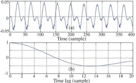
we took a frame (400 samples) of an =i:= sound signal recorded from a female speaker and computed its correlation coefficients cx;l,l¼0;1;…;20, using a short-time average. Both the waveform and correlation coefficients are plotted in Fig.1. Using these estimated correlation coefficients and set-ting the parameter L to 20, we performed the orthogonal decomposition of the =i:=sound signal xðkÞ. The first and second coefficients ofxdðkÞandx0ðkÞas a function of timek

are shown in Fig. 2. Sincecx;0¼1, we havexd;0ðkÞ ¼xðkÞ

andx00ðkÞ ¼0, which can be seen from Figs.2(a)and2(b).

But aslincreases, the correlation betweenxðkÞandxðklÞ

decreases, and as a result, the level ofxd;lðkÞdecreases while that of x0_lðkÞ increases, which can be seen by comparing Figs.2(a)with2(c)and2(b)with2(d). Figures2(c)and2(d) show xd;1ðkÞ and x01ðkÞ. Note that in practice cx cannot be computed directly since xðkÞ is not accessible. However, slightly rearranging(17), we get

c_x¼E½yðkÞyðkÞ E½vðkÞ

vðkÞ E½y2_{ðkÞ E½v}2_ðkÞ ¼

r2

ycyr2vcv

r2

yr2v

; (19)

where r2

y¼D E½y2ðkÞand r2v¼

D _E½v2_{ðkÞ are the variances of}

yðkÞandvðkÞ, respectively. One can see that now_c

xdepends on the statistics ofyðkÞandvðkÞ. The statistics ofyðkÞcan be computed directly sinceyðkÞis accessible while the statistics ofvðkÞcan be estimated based on the use of a voice activity detector (VAD) (Cohenet al., 2010).

Now substituting(14)into(5), we get

^

xðkÞ ¼hTxdðkÞ þhTx0ðkÞ þhTvðkÞ: (20)

Since it is correlated with the desired signal samplexðkÞ, the vectorxdðkÞwill help estimatexðkÞ. So, the first term on the

FIG. 1. (Color online) A frame of an =i:=sound signal recorded from a

right-hand side of (20) is clearly the filtered desired signal and we denote it asxfdðkÞ ¼D hTxdðkÞ ¼xðkÞhTc_x. In

compar-ison,x0_{ðkÞis orthogonal toxðkÞ; so this vector would}

inter-fere with the estimation. Therefore, we introduce the term “interference,” defined asx0

riðkÞ ¼D hTx0ðkÞ. The third term on

the right-hand side of (20) is the residual noise, as in the classical approaches, i.e.,v_rnðkÞ ¼D hTvðkÞ. So, the signal esti-mate can now be written as

^

xðkÞ ¼xfdðkÞ þxri0ðkÞ þvrnðkÞ: (21)

It can be checked that the three terms xfdðkÞ, x0riðkÞ, and

v_rnðkÞare mutually uncorrelated. Therefore, the variance of

^

xðkÞis

r2 ^

x¼r

2

xfdþr 2

x0 riþr

2

v_rn; (22)

where

r2_xfd ¼r2_xðhT

c_xÞ2¼hTRxdh; (23)

r2_x0 ri ¼h

T_R

x0h¼hTR_xhr2_xðhTc_xÞ2; (24)

r2v_rn ¼h

T_R

vh; (25)

r2

x¼D E½x2ðkÞ is the variance of xðkÞ, Rxd ¼r 2

xcxcTx is the correlation matrix (whose rank is equal to 1) of xdðkÞ, and Rx0¼D E½x0ðkÞx0TðkÞis the correlation matrix ofx0ðkÞ.

With the above decomposition, one can see that the objective of noise reduction is to find a good filter that makes xfdðkÞas close as possible toxðkÞand meanwhile minimizes

the effect of bothx0_riðkÞandv_rnðkÞ. To find such a filter, we first define the error signal between the estimated and desired signals as

eðkÞ ¼Dx^ðkÞ xðkÞ ¼edðkÞ þerðkÞ; (26)

where

edðkÞ ¼DxfdðkÞ xðkÞ (27)

is the signal distortion due to the FIR filter and

erðkÞ ¼Dx0riðkÞ þvrnðkÞ (28)

represents the residual interference-plus-noise. The MSE is then

JðhÞ ¼E½e2ðkÞ ¼JdðhÞ þJrðhÞ; (29)

where

JdðhÞ ¼E½e2dðkÞ ¼r 2

xðhTcx1Þ

2

(30)

and

JrðhÞ ¼E½e2rðkÞ ¼r 2

x0 riþr

2

v_rn: (31)

Comparing(26)with(7)and(29)with(11), one can clearly see the difference between the new definitions of the error signal and MSE in our new model and the traditional defini-tions. It is clear that the objective of noise reduction with the new linear model is to find optimal FIR filters that would ei-ther minimize JðhÞ or minimize JrðhÞ or JdðhÞ subject to

some constraint. But before deriving the optimal filters, we first give some very useful measures that fit well with the new linear model.

V. PERFORMANCE MEASURES

Many distance measures have been developed to evalu-ate noise reduction, such as the Itakura distance, the Itakura-Saito distance (ISD) [that performs a comparison of spectral envelopes (AR parameters) between the clean and the proc-essed speech] (Itakura and Saito, 1970;Quackenbushet al., 1988;Chenet al., 2003), SNR, speech distortion index, noise reduction factor (Benestyet al., 2009; Benestyet al., 2005; Chenet al., 2006), etc. Many of these measures are defined based on the classical linear filter model. As it was shown in the previous section, the filtered speech (where the desired signal does not appear explicitly) should be separated into the filtered desired speech and interference. The interference part interferes with the estimation of the desired speech sig-nal and it should be treated as part of the noise. Therefore, it is necessary to redefine some of the performance measures originally established for the classical model.

The first measure is the input SNR defined as

iSNR¼r 2

x r2 v

: (32)

FIG. 2. (Color online) The orthogonal decomposition of the signal in Fig.1:

To quantify the level of noise remaining at the output of the filter, we define the output SNR as the ratio of the variance of the filtered desired signal over the variance of the residual interference-plus-noise (in this paper, we consider the inter-ference as part of the noise in the definitions of the perform-ance measures since it is uncorrelated with the desired signal), i.e.,

is the interference-plus-noise correlation matrix. The objec-tive of the noise reduction filter is to make the output SNR greater than the input SNR so that the quality of the noisy signal will be enhanced. For the particular filter h¼i0,

wherei0 is the first column of the identity matrix I(of size

LL), we have

oSNRði0Þ ¼iSNR: (35)

Now, let us define the quantity

oSNRmax¼DkmaxðR1in RxdÞ; (36)

where kmaxðR1in RxdÞ denotes the maximum eigenvalue of

the matrixR1in Rxd. Since the rank of the matrixRxdis equal

where tr½ denotes the trace of a square matrix. It can be checked that the quantity oSNRmaxcorresponds to the

maxi-mum SNR that can be achieved through filtering since the filter,hmax, that maximizes oSNRðhÞ[Eq.(33)] is the

eigen-vector corresponding to the maximum eigenvalue of

R1in Rxd. As a result, we have

oSNRðhÞ oSNRmax; 8h (38)

and

oSNRmax¼oSNRðhmaxÞ oSNRði0Þ ¼iSNR: (39)

The noise reduction factor (Benestyet al., 2005;Chenet al., 2006) quantifies the amount of noise that is rejected by the filter. This quantity is defined as the ratio of the variance of the noise at the microphone over the variance of the interfer-ence-plus-noise remaining after the filtering operation, i.e.,

nnrðhÞ ¼D

The noise reduction factor is expected to be lower bounded by 1 for optimal filters.

In practice, the FIR filter,h, distorts the desired signal. In order to evaluate the level of this distortion, we define the speech reduction factor (Benestyet al., 2009) as the variance of the desired signal over the variance of the filtered desired signal at the output of the filter, i.e.,

nsrðhÞ ¼

An important observation is that the design of a filter that does not distort the desired signal requires the constraint

hT

c_x¼1: (42)

Thus, the speech reduction factor is equal to 1 if there is no distortion and expected to be greater than 1 when distortion occurs.

By making the appropriate substitutions, one can derive the relationship among the four previous measures:

oSNRðhÞ

iSNR ¼ nnrðhÞ

nsrðhÞ

: (43)

When no distortion occurs, the gain in SNR coincides with the noise reduction factor.

Another useful performance measure is the speech dis-tortion index (Benesty et al., 2005; Chen et al., 2006)

The speech distortion index is always greater than or equal to 0 and should be upper bounded by 1 for optimal filters; so the higher is the value ofv_sdðhÞ, the more the desired signal is distorted.

VI. OPTIMAL FILTERS

We have defined the MSE criterion with the new linear model in Sec.IV. For the particular filterh¼i0, the MSE is

Jði0Þ ¼r2v: (45)

In this case, there is neither noise reduction nor speech dis-tortion. We can now define the normalized MSE (NMSE) as

This shows how the MSEs are related to some of the per-formance measures.

It is clear that the objective of noise reduction with the new linear model is to find optimal FIR filters that would ei-ther minimize JðhÞ or minimize JrðhÞ or JdðhÞ subject to

some constraint. In this section, we derive three fundamental filters with the revisited linear model and show that they are fundamentally equivalent. We also show their equivalence withhmax(i.e., the maximum SNR filter).

A. Wiener

The Wiener filter is easily derived by taking the gradient of the MSE, i.e.,JðhÞdefined in(29), with respect tohand equating the result to zero:

hW¼R1y Rxi0¼ ½IR1y Rvi0: (49)

Since

Rxi0¼r2_xc_x; (50)

we can rewrite(49)as

hW¼r2_xR1_y c_x: (51)

From Sec.IV, it is easy to verify that

Ry¼r2xcxcTxþRin: (52)

Determining the inverse of Ry from(52) with Woodbury’s

identity

and substituting the result into(51), we get another interest-ing formulation of the Wiener filter:

hW¼

R1in cx r2

x þcTxR1in cx

; (54)

that we can rewrite as

hW¼

Using(54), we deduce that the output SNR is

oSNRðhWÞ ¼oSNRmax¼tr½R1in Ry L; (56)

and the speech distortion index is a clear function of the maximum output SNR:

v_sdðh_WÞ ¼ 1

ð1þoSNRmaxÞ

2: (57)

The higher is the value of oSNRmax, the less the desired

sig-nal is distorted.

Since the Wiener filter maximizes the output SNR according to(56), we have

oSNRðhWÞ oSNRði0Þ ¼iSNR: (58)

It is interesting to see that the two filters hW andhmax both

maximize the output SNR. So, they are equivalent (different only by a scaling factor).

With the Wiener filter the noise reduction factor is

nnrðhWÞ ¼

Using (57) and (59) in (46), we find the minimum NMSE (MNMSE):

The celebrated MVDR filter proposed by Capon

(Capon, 1969) is usually derived in a context where we have

at least two sensors (or microphones) available. Interest-ingly, with the new linear model, we can also derive the MVDR (with one sensor only) by minimizing the MSE of the residual interference-plus-noise, JrðhÞ, with the

con-straint that the desired signal is not distorted. Mathemati-cally, this is equivalent to

min

h h

T_R

inh subject to hTc_x¼1: (61)

The solution to the above optimization problem is

hMVDR¼ R1in cx

cT_xR1_in c_x

; (62)

which can also be written as

hMVDR¼

Obviously, we can rewrite the MVDR as

hMVDR¼ R1y cx

cT_xR1_y c_x

: (64)

The Wiener and MVDR filters are simply related as follows

So, the two filtershWandhMVDRare equivalent up to a

scal-ing factor. From a theoretical point of view, this scalscal-ing is not significant. But from a practical point of view it can be important. Indeed, the signals are usually nonstationary and the estimations are done on a frame-by-frame basis, so it is essential to have this scaling factor right from one frame to another in order to avoid large distortions. Therefore, it is recommended to use the MVDR filter rather than the Wiener filter in speech enhancement applications.

Locally, a scaling factor should not affect the SNR, but it can change the level of speech distortion and noise reduc-tion. We should have

However, from a global viewpoint, the time-varying scaling factor may put more attenuation in silence periods where the desired speech is absent and less attenuation when speech is present. This weighting process can cause some performance differences between the MVDR and Wiener filters if the per-formance is evaluated on a long-term basis. We will come back to this point when we discuss the experiments.

C. Tradeoff

In the tradeoff approach, we try to compromise between noise reduction and speech distortion. Instead of minimizing the MSE as we already did to find the Wiener filter, we could minimize the speech distortion index with the constraint that the noise reduction factor is equal to a positive value that is greater than 1. Mathematically, this is equivalent to

min

h JdðhÞ subject to JrðhÞ ¼br

2

v; (72)

where 0<b<1 to insure that we get some noise reduction. By using a Lagrange multiplier, l0, to adjoin the con-straint to the cost function, we easily deduce the tradeoff filter: we get the MVDR filter. Withl, we can make a compromise between noise reduction and speech distortion. Again, we observe here as well that the tradeoff and Wiener filters are

equivalent up to a scaling factor. Locally at each time instant k, the scaling factor should not affect the SNR. So, the output SNR of the tradeoff filter is independent ofland is identical to the output SNR of the Wiener filter, i.e.,

oSNRðhT;lÞ ¼oSNRðhWÞ; 8l: (74)

VII. THE LCMV FILTER

We can derive an LCMV filter (Frost, 1972;Er and

Can-toni, 1983) which can handle more than one linear

con-straint, by exploiting the structure of the noise signal. In Sec.IV, we decomposed the vectorxðkÞinto two or-thogonal components to extract the desired signal,xðkÞ. We can also decompose (but not for the same reason) the noise signal vector,vðkÞ, into two orthogonal vectors:

vðkÞ ¼vðkÞc

Our problem this time is the following. We wish to per-fectly recover our desired signal, xðkÞ, and completely remove the correlated components, vðkÞc

v. Thus, the two

constraints can be put together in a matrix form as

CTh¼i; (76)

where

C¼ ½cxcv (77)

is our constraint matrix of sizeL2 and

i¼ ½1 0T:

Then, our optimal filter is obtained by minimizing the energy at the filter output, with the constraints that the correlated noise components are cancelled and the desired speech is preserved, i.e.,

hLCMV¼arg min

h h

T_R

yh subject to CTh¼i: (78)

The solution to(78)is given by

hLCMV¼R1y C½CTR1y C

1

i: (79)

By developing(79), it can easily be shown that the LCMV can be written as a function of the MVDR:

t¼ R becomes the MVDR filter; however, when q2

tends to 1, which happens if and only if c_x¼cv, we have no solution

since we have conflicting requirements. Obviously, we always have

The LCMV filter is able to remove all the correlated noise but at the price that its overall noise reduction is lower than that of the MVDR filter.

VIII. EXPERIMENTAL RESULTS

We have redefined the error signals, optimization cost functions, and evaluation criteria for the noise reduction problem in the time domain and derived several new optimal noise reduction filters. In this section, we study those filters through experiments.

The clean speech signal used in our experiments was recorded from a female speaker in a quiet office room. It was originally sampled at 16 kHz and then downsampled to 8 kHz. The overall length of the signal is approximately 10 min, but only the first 30 s is used in our experiments. Noisy speech is obtained by adding noise to the clean speech (the noise signal is properly scaled to control the input SNR level). We consider three types of noise: a white Gaussian random process, a babble noise signal recorded in a New York Stock Exchange (NYSE) room, and a competing speech signal recorded from a male speaker. The NYSE noise and the competing speech signal were also digitized with a sampling rate of 16 kHz, but again they were down-sampled into 8 kHz. Compared with Gaussian random noise which is stationary and white, the NYSE noise is nonstation-ary and colored. It consists of sounds from various sources such as electrical fans, telephone rings, and background speech. SeeHuanget al.(2008)for a more detailed descrip-tion of this babble noise. The male interference speech signal will be used to evaluate the LCMV filter for its performance in reducing correlated noise.

A. Estimation of correlation matrices and vectors

The implementation of most of the noise reduction filters derived in Secs.VIandVIIrequires the estimation of the cor-relation matrices Ry,Rx, and Rv, the correlation vector cx,

and the signal variance r2

x. Computation of Ry is relatively

easy because the noisy signalyðkÞis accessible. But in

prac-tice, we need a noise estimator or a VAD to compute all the other parameters. The problems regarding noise estimation and VAD have been widely studied in the literature and we have developed a recursive algorithm in our previous research that can achieve reasonably good noise estimation in practical environments (Chenet al., 2006). However, in this paper, we will focus on illustrating the basic ideas while set-ting aside the noise estimation issues. So, we will not use any noise estimator in the following experiments. Instead, we directly compute the noise statistics from the noise signal. Specifically, at each time instantk, the matrixRy (its size is

in the range between 44 and 8080) is computed using the most recent 400 samples (50 ms long) of the noisy signal with a short-time average. The matrix Rv is also computed

using a short-time average; but noise is in general stationary (except for the competing speech case whereRy andRv are

computed in the same way), so we use 640 samples (80 ms long) to compute Rv. Then the R^x matrix is computed

according toR^x¼R^yR^v, and^c_xis calculated using(19).

B. Comparison between the traditional and new performance measures

In this experiment, we compare the traditional perform-ance measures defined based on the filtered speech xfðkÞ

with the new performance measures defined using the fil-tered desired signalxfdðkÞand interferencex0riðkÞ. The

Wie-ner filter given in (51)is used in this experiment, which is the same for both the traditional definition of the error signal shown in(7) and the new decomposition of the error signal given in (26) (since the Wiener filter minimizes the overall MSE, which is not affected by any decomposition form of the error signal). Specifically, at each time instantk, we first compute the correlation matrixR^y, the correlation vector^c_x,

and the signal variance^r2_x as described in the previous sub-section. A Wiener filter is then constructed according to (51). Applying this Wiener filter toyðkÞ,xðkÞ, andvðkÞ, we obtain the enhanced signalx^ðkÞ, the filtered signalxfðkÞ, the

filtered desired signal xfdðkÞ, the interferencex0riðkÞ, and the

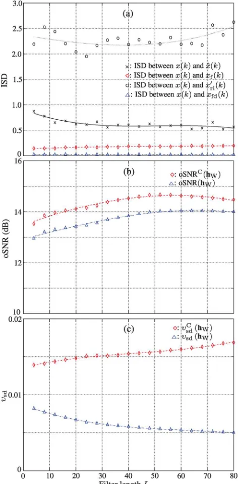
residual noisev_rnðkÞ. To illustrate the importance of separat-ing the filtered signal into the filtered desired signal and in-terference, we computed the ISDs between the clean speech xðkÞ and the signalsx^ðkÞ, xfðkÞ,xfdðkÞ, and x0riðkÞ obtained

with the Wiener filter. The results as a function of the filter lengthLfor the white Gaussian noise case with iSNR¼10 dB are plotted in Fig. 3(a). It is seen that the ISD between the clean speechxðkÞand the filtered desired signalxfdðkÞis

approximately 0, indicating that these two signals are almost the same. In comparison, the ISD betweenxðkÞandx0_riðkÞis very large, which shows that these two signals are signifi-cantly different in spectrum. Therefore, x0

riðkÞshould not be

treated as part of the desired signal after filtering, which veri-fies the necessity of separating the filtered signal into the fil-tered desired signal and residual interference. The ISD between the clean speech and the filtered signal xfðkÞ is

larger than that between the clean speech and the filtered desired signal xfdðkÞ; but it is significantly smaller than the

ISD between xðkÞ and x0_riðkÞ. This shows thatxfdðkÞ is the

much lower than that of xfdðkÞ, which is desired in noise

reduction. It is noticed that the filter lengthLdoes not affect much the ISD betweenxðkÞandxfdðkÞ. But the ISD between

xðkÞ and xfðkÞ slightly increases with L. This variation is

mainly caused by the residual interference. The ISD between the clean speech and its estimate, ^xðkÞ, first decreases asL increases up to 30; but it does not change much if we further increase L. This confirms the results reported inChenet al.

(2006) and indicates that for the time-domain Wiener filter

with an 8 kHz sampling rate, 30 is a sufficient filter length and, a larger length will not significantly improve the speech quality but would dramatically increase the complexity of the algorithm.

With the new decomposition of the error signal, the out-put SNR [given in(33)] is defined as the ratio of the intensity of the filtered desired signal over the intensity of the residual interference-plus-noise. Traditionally, however, the whole filtered signalxfðkÞis treated as the desired signal after noise

reduction, so the output SNR of the Wiener filter is in the following form

oSNRCðhWÞ ¼

r2

xf

r2 v_rn

; (87)

where, again, we use the superscriptC to indicate the “classical” definition. Both oSNRðhWÞand oSNRCðhWÞare

plotted in Fig. 3(b)as a function of the filter length L. The trends between the two versions of the output SNR and the filter length L are similar. But the new definition should be more accurate as the residual interference is not treated as part of the desired speech signal.

Also plotted in Fig. 3 is the speech distortion index defined in (44). For the purpose of comparison, we also showed the “classical” definition of this index, which is given by

vC

sdðhWÞ ¼

Ef½xfðkÞ xðkÞ2g

r2

x

: (88)

It is seen that v_sdðh_WÞdecreases withL(rapidly for smallL values). But with the classical definition, the speech distor-tion index increases with L, which is similar to the ISD betweenxðkÞandxfðkÞin Fig.3(a). This difference between

the two indices is due to the residual interference.

We also studied the case of the NYSE babble noise. The results are shown in Fig.4. Again, the appropriateness of the new performance measures is verified.

C. Comparison between the Wiener and MVDR filters

With the new decomposition of the error signal, we have shown that it is now possible to derive an MVDR filter for single-channel noise reduction. The difference between the MVDR and Wiener filters is a scaling factor, which is given in(66). If this scaling factor is time-invariant, the Wie-ner and MVDR filters have the same performance. However, in speech applications, the desired speech signal is always nonstationary and noise statistics may change with time. As a result, the scaling factor is in general time-varying, which can cause some performance difference between the two fil-ters. This subsection studies the difference between the MVDR and Wiener filters through experiments. Based on the previous experiment, we set the filter length L to 20. White Gaussian noise is used and the correlation matrixR^y

is computed using the method described in Sec. VIII A. However, unlike the previous experiment, here we directly compute^c_xand^r2_x from the signalxðkÞusing a same

short-time average as R^y. We then estimate the scaling factor

between the MVDR and Wiener filters according to (66). The first 3 s of the noisy speech (with iSNR¼10 dB) and the computed scaling factor are plotted in Fig.5(in both the linear and dB scales). It is seen that the value of the scaling

FIG. 3. (Color online) Comparison between the traditional performance

measures [based on xfðkÞ and the new performance measures [based on

xfdðkÞandx0riðkÞwith the Wiener filter. The white Gaussian noise is used

factor is large (close to 1) during the presence of speech; but it is very small (close to 0) in silence periods. Figure 5(d) plots the noisy speech multiplied with the scaling factor. It is seen that the noise in silence periods is significantly attenu-ated while the noise level in the presence of speech remains almost unchanged. This indicates that the Wiener filter is more aggressive in suppressing silence periods while it behaves almost the same as the MVDR filter during the pres-ence of speech.

The performance results for this experiment are sketched in Fig.6. One can notice that speech distortion either meas-ured by the ISD or by the speech distortion index is zero with

the MVDR filter. When the SNR is above 15 dB, the MVDR and Wiener filters have almost the same performance. How-ever, as the SNR decreases, the Wiener filter tends to have more noise reduction, but it has more speech distortion as well. It should be noted that all the performance measures shown in Fig.6are computed globally with the use of all the signal samples. If we evaluate the measures on a short-time basis, the two filters would have similar output SNRs during the presence of speech. The reason that the Wiener filter achieves a higher global output SNR is that it suppresses more noise during the absence of speech. This, however, causes some discontinuity in the residual noise level, which is unpleasant to listen to and should be avoided in practice.

Experiments using the NYSE noise were also conducted and the performance difference between the two filters is similar to that in the white Gaussian noise case.

D. The tradeoff filter

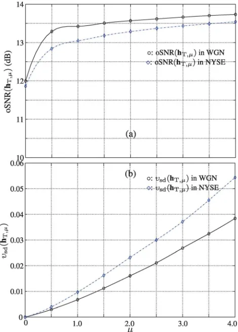
The tradeoff filter derived in Sec.VI Cintroduces a non-negative parameter l to control the residual noise level. Whenl¼0, the tradeoff filter degenerates to the MVDR fil-ter. This experiment is to investigate the effect of l on the output SNR and speech distortion. Similar to the MVDR and Wiener filters, we need to know the matrixR^y, the vector^c_x,

and the signal variancer^2_x. Again, these parameters are com-puted using the method described in Sec.VIII A. The results for both the white Gaussian and NYSE noise cases are shown in Fig. 7. It is seen that both the output SNR and speech distortion index increase aslincreases. Theoretically at each time instantk, increasinglshould not affect the out-put SNR. But the value of the parameter l controls how

FIG. 4. (Color online) Comparison between the traditional performance

measures [based on xfðkÞ and the new performance measures [based on

xfdðkÞandx0riðkÞwith the Wiener filter. The NYSE noise is used and the

input SNR is 10 dB.

FIG. 5. (Color online) (a) The clean speech waveform, (b) the noisy speech

waveform, (c) the scaling factorabetween the Wiener and MVDR filters

given in(66), (d) the scaling factor in the dB scale, and (e) the noisy speech

multiplied by the scaling factor. The white Gaussian noise is used with

aggressive the filter suppresses silence periods where the desired speech is absent. A larger value of l indicates that the filter is more aggressive in suppressing silence periods. So, when we evaluate the output SNR globally, we have more SNR gain for a larger value ofl.

It is noticed that in the NYSE noise case, the output SNR is lower and the speech distortion index is larger. This is due to the fact that this noise is nonstationary and, hence, more difficult to deal with than with the white Gaussian noise.

E. The LCMV filter

The LCMV filter is derived based on the constraints that the desired speech ought to be perfectly recovered while the

correlated components in noise (if any) should be removed. In other words, the LCMV filter needs to meet two constraints simultaneously, i.e.,cT_xh¼1 andcTvh¼0. Consequently, the

filter length of the LCMV filter should be much longer than that of the MVDR filter since the latter only needs to satisfy

cT_xh¼1 while minimizing the interference-plus-noise. The

performance of the LCMV filter depends not only on the filter length, but also on the degree of speech and noise self correla-tion. In this experiment, we investigate the LCMV filter in three different noise backgrounds: white Gaussian noise, NYSE noise, and speech from a competing talker. In the first case, the noise samples are completely uncorrelated. There-fore, we havecv¼i0. Forcingc

T

vh¼0 in this case meansh0

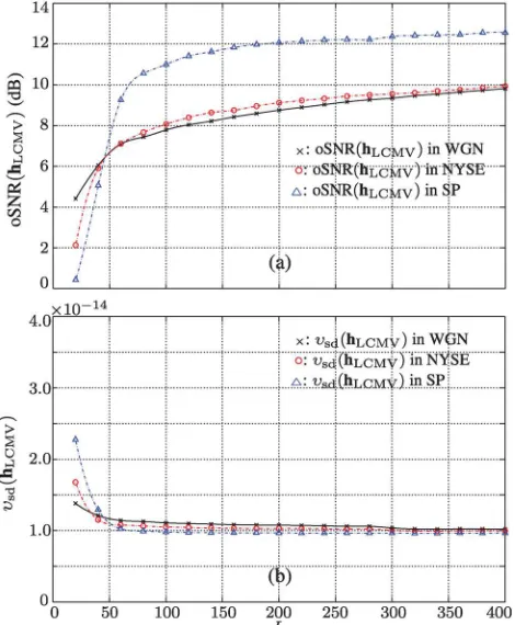
should be 0, which implies that the current speech sample xðkÞis completely predicted from the previousL1 samples. In the NYSE noise case, there will be some but weak correla-tion among neighboring samples, while in the competing speech case, the correlation between signal samples can be very strong. The results of this experiment are shown in Fig. 8. The input SNR is 10 dB, and again the noisy correla-tion matrix and the speech and noise correlacorrela-tion vectors are directly computed from the noisy, clean, and noise signals. It is seen that the speech distortion index in the three conditions is very small (of the order of 1014), indicating that the desired speech signal is estimated without speech distortion. The output SNR in three conditions increases with the filter length L. WhenL is reasonably large (>50), slightly more SNR gain is achieved in the NYSE noise case than in the

FIG. 6. (Color online) Comparison between the Wiener and MVDR filters

in the white Gaussian noise case withL¼20.

FIG. 7. (Color online) Performance of the tradeoff filter as a function ofl.

white Gaussian noise case, while the output SNR for the com-peting speech situation is significantly higher than those in the NYSE and Gaussian noise cases. This coincides with the the-oretical analysis that the LCMV is designed to remove corre-lated components in noise. The stronger the noise self correlation, the higher the SNR improvement.

It is also noticed that for the white Gaussian and NYSE noise cases, the output SNR is lower than the input SNR. This indicates that the LCMV filter boosts the uncorrelated components of noise while removing its correlated compo-nents. This problem is more serious when the filter length is short. One way to circumvent this issue is to put a penalty term in the cost function so as the filter does not amplify the uncorrelated noise components, i.e.,

hLCMV¼arg min

h ðh

T_R

yhþdhThÞ subject to CTh¼i;

(89)

wheredis a positive constant that controls how strongly we impose the penalty. The solution to(89)is given by

hLCMV¼ ðRyþdIÞ1C½CTðRyþdIÞ1C1i: (90)

Comparing(90)with(79), one can see that adding a penalty term is identical to putting a regularization parameter when computing the inverse of the noisy correlation matrix. By choosing a proper value of this regularization, the LCMV fil-ter can be more robust to the uncorrelated noise component. But we should note that, unlike the MVDR filter, the LCMV is not designed to reduce the self uncorrelated noise. So, no matter how we control the regularization factor, we should not expect much SNR improvement if the noise is white.

IX. CONCLUSIONS

This paper studied the noise reduction problem in the time domain. We presented a new way to decompose the clean speech vector into two orthogonal components: one is correlated and the other is uncorrelated with the current clean speech sample. While the correlated component helps estimate the clean speech, the uncorrelated component inter-feres with the estimation, just as the additive noise. With this new decomposition, we discussed how to redefine the error signal and form different cost functions and addressed the issue of how to design different optimal noise reduction filters by optimizing these new cost functions. We showed that with the redefined error signal, the maximum SNR filter is equivalent to the widely known Wiener filter. We demon-strated that it is possible to derive an MVDR filter that can reduce noise without adding any speech distortion in the single-channel case. This new MVDR filter is different from the Wiener filter only by a scaling factor, where by adjust-ing this scaladjust-ing factor, the Wiener filter tends to be more aggressive in suppressing noise during silence periods, which can cause significant discontinuity in the residual noise level that is unpleasant to listen to. We also showed that an LCMV filter can be developed to remove correlated components in noise without adding distortion to the desired speech signal. Furthermore, several performance measures have been defined based on the new orthogonal decomposi-tion of the clean speech vector, which are more appropriate than the traditional ones for the evaluation of the noise reduction filters.

Benesty, J., Chen, J., Huang, Y., and Cohen, I. (2009). Noise

Reduc-tion in Speech Processing (Springer-Verlag, Berlin), pp. 1–229. Benesty, J., Chen, J., Huang, Y., and Doclo, S. (2005). “Study of the

wiener filter for noise reduction,” inSpeech Enhancement, edited by J.

Benesty, S. Makino, and J. Chen (Springer-Verlag, Berlin), Chap. 2, pp. 9–41.

Boll, S. F. (1979). “Suppression of acoustic noise in speech using spectral

subtraction,” IEEE Trans. Acoust., Speech, Signal Process. ASSP-27,

113–120.

Capon, J. (1969). “High resolution frequency-wavenumber spectrum

analy-sis,” Proc. IEEE57, 1408–1418.

Chen, G., Koh, S. N., and Soon, I. Y. (2003). “Enhanced itakura measure incorporating masking properties of human auditory system,” Signal

Pro-cess.83, 1445–1456.

Chen, J., Benesty, J., and Huang, Y. (2009). “Study of the noise-reduction problem in the karhunen-loe`ve expansion domain,” IEEE Trans. Audio,

Speech, Language Process.17, 787–802.

Chen, J., Benesty, J., Huang, Y., and Doclo, S. (2006). “New insights into the noise reduction wiener filter,” IEEE Trans. Audio, Speech, Language

Process.14, 1218–1234.

Cohen, I., Benesty, J., and Gannot, S., eds. (2010).Speech Processing in

Modern Communication–Challenges and Perspectives(Springer, Berlin), pp. 1–342.

Ephraim, Y., and Malah, D. (1984). “Speech enhancement using a

minimum-mean square error short-time spectral amplitude

estimator,” IEEE Trans. Acoust., Speech, Signal Process. ASSP-32,

1109–1121.

Er, M., and Cantoni, A. (1983). “Derivative constraints for broad-band ele-ment space antenna array processors,” IEEE Trans. Acoust., Speech,

Sig-nal Process.31, 1378–1393.

Frost, O. (1972). “An algorithm for linearly constrained adaptive array

proc-essing” Proc. IEEE60, 926–935.

Huang, Y., Benesty, J., and Chen, J. (2008). “Analysis and comparison of multichannel noise reduction methods in a common framework,” IEEE

Trans. Audio, Speech, Language Process.16, 957–968.

FIG. 8. (Color online) Performance of the LCMV filter as a function ofLin

Itakura, F., and Saito, S. (1970). “A statistical method for estimation of speech spectral density and formant frequencies,” Electron. Commun. Ja-pan53A, 36–43.

Loizou, P. (2007).Speech Enhancement: Theory and Practice(CRC Press,

Boca Raton, FL), pp. 1–585.

Martin, R. (2001). “Noise power spectral density estimation based on opti-mal smoothing and minimum statistics,” IEEE Trans. Speech, Audio

Pro-cess.9, 504–512.

Quackenbush, S. R., Barnwell, T. P., and Clements, M. A. (1988).Objective

Measures of Speech Quality (Prentice-Hall, Englewood Cliffs, NJ), pp. 1–355.

Vary, P. (1985). “Noise suppression by spectral magnitude estimation–

mechanism and theoretical limits,” Signal Process.8, 387–400.

Vary, P., and Martin, R. (2006). Digital Speech Transmission:

Enhance-ment, Coding and Error Concealment(John Wiley and Sons, Chichester, England), pp. 1–625.

464 J. Acoust. Soc. Am., Vol. 132, No. 1, July 2012 Benestyet al._{: Time-domain noise reduction}