Modeling 3D Wings Like Object Based On Finite-Different Time-Domain (FDTD) Method In Graphical User Interface For Radar Cross Section (RCS).

Modeling 3D Wings Like Object Based On Finite-Different Time-Domain (FDTD) Method In Graphical User Interface For Radar Cross Section (RCS)

NAZRUL AFFENDI BIN CHE IBRAHIM

This Report Is Submitted In Partial Fulfillment Of Requirements For The Bachelor Degree of Electronic Engineering (Electronic Telecommunication)

Fakulti Kejuruteraan Elektronik dan Kejuruteraan Komputer Universiti Teknikal Malaysia Melaka

v

vi

ACKNOWLEDGEMENT

Alhamdulillah for His Blessing, finally I have completed my Final Year Project for Bachelor Degree of Electronic Engineering (Telecommunication). Here I would like to thank for several people to involving in making this project successful. Without them, I would much difficult to accomplish the objectives of this project.

First of all, I would like to express deepest appreciation to my supervisor En Fauzi Bin Mohd Johar for assistance and guidance towards the progress of this project. Besides that, with his lecture, offering encouragement and been patiently monitoring my progress to complete my project. ”. Obviously the progress I had now will be uncertain without her assistance. I would like very thanks again to him.

vii

ABSTRACT

viii

ABSTRAK

ix

LIST OF FIGURE

CHAPTER TITLE PAGE

PROJECT TITLE i

REPORT STATUS VERIFICATION FORM ii

STUDENT’S DECLARATION iii

SUPERVISOR’S DECLARATION iv

ACKNOWLEDGEMENT vi

ABSTRACT (ENGLISH) vii

ABSTRAK (MALAY) viii

TABLE OF CONTENT ix

LIST OF FIGURE xvi

LIST OF TABLE xvii

LIST OF ABBREVIATIONS xviii

I INTRODUCTION

1.1 OVERVIEW 1

1.2 OBJECTIVE 2

1.3 PROBLEM STATEMENT 3

1.4 SCOPE OF PROJECT 4

1.4.1 Understanding FDTD Algorithm 4

1.4.2 Design object in FDTD 6

x

1.4.4 Simulate using FDTD with Graphical User

Interfaces (GUI) 7

II LITERATURE REVIEW

2.1 CLASSIFICATION OF METHOD OF ANALYSIS 8 2.2 FINITE DIFERRENT TIME- DOMAIN (FDTD) 11

2.2.1 Basic Principles FDTD 11

2.2.2 Boundary Condition 27

2.2.3 Near Field Far Field Transformation 29

III RADAR CROSS SECTION (RCS)

3.1 DEFINITION OF RADAR CROSS SECTION 32 3.2 FACTOR AFFECTING PERFORMANCE OF

RADAR CROSS SECTION 33

3.2.1 Material Object Made 33

3.2.2 Size or Shape of Object Target 34 3.2.3 Polarization and Incident Angle Plane Wave 35

IV METHODOLOGY

4.1 FLOW CHART OF IMPLEMENTATION

PLANNING 37

4.2 FLOW CHART OF FDTD PROGRAM 39

4.3 SOFTWARE DESIGN 41

V RESULT AND ANALYSIS

5.1 INTRODUCTION 43

5.2 PROJECT RESULT IN GRAPHICAL USER

INTERFACE 44

5.3 ANALYSIS OF RCS PATTERN BASED ON

INCIDENT ANGLE PLANE WAVE 45

xi

5.3.2 Analyze at B-Direction of Incident Angle 49 5.3.3 Analyze at C-Direction of Incident Angle 51 5.3.4 Analyze at D-Direction of Incident Angle 53 5.4 ANALYZE RCS PATTERN BASED ON TYPES OF

OBJECT 56

VI CONCLUSION AND SUGGESTION

6.1 INTRODUCTION 59

6.2 CONCLUSION 59

6.3 SUGGESTION AND FUTURE WORKS 61

REFERENCE 62

xii

LIST OF FIGURE

FIGURE TITLE PAGE

1.1 Yee unit cell in 3 Dimension. 5

1.2 Top view measurement of wing-shaped. 6 1.3 Side view measurement of wing-shaped. 6

1.4 MATLAB Software. 7

2.1 Classification of Method for Analysis. 10 2.2 The FDTD unit cell as proposed by Yee. 16 2.3 Approximation of derivative of f(x) at x by finite difference:

central differences. 17

2.4 An FDTD problem space and the objects approximated by

snapping to cells. 18

2.5 Arrangement of field components on a Yee cell index. 18 2.6 The three-dimensional problem space is truncated by

absorbing boundaries. 27

2.7 The CPML on the plane boundary. 28

2.8 An imaginary surface is selected to enclose the antennas or

scatters. 30

2.9 Equivalent surface currents on the imaginary closed surface. 30 3.1 Reflection Signal and RCS Pattern with shaping object 34

3.2 Radar and frequency band. 35

3.3 The Rectangular coordinate with the origin

xiii

4.1 Flow chart overall planning. 38

4.2 Flow Chart of FDTD Overall Program. 39

4.3 MATLAB Software. 41

4.4 RCS Pattern in GUI Matlab. 42

5.1 Main Page of GUI Project. 44

5.2 Intro Page of GUI Project. 44

5.3 Overview Page of GUI Project. 44

5.4 Simulation Page of GUI Project. 44

5.5 Direction of Angle Incident Wave. 45 5.6 RCS Pattern for Plane XY at frequency 10 GHz (Blue) and

15 GHz (Red) in Phi-Data.(A- Direction Incident Angle) 46 5.7 RCS Pattern for Plane XZ at frequency 10 GHz (Blue) and

15 GHz (Red) in Phi-Data. (A- Direction Incident Angle) 46 5.8 RCS Pattern for Plane YZ at frequency 10 GHz (Blue) and

15 GHz (Red) in Phi-Data. (A- Direction Incident Angle) 47 5.9 RCS Pattern for Plane XY at frequency 10 GHz (Blue) and

15 GHz (Red) in Theta-Data. (A- Direction Incident Angle) 47 5.10 RCS Pattern for Plane XZ at frequency 10 GHz (Blue) and

15 GHz (Red) in Theta-Data. (A- Direction Incident Angle) 47 5.11 RCS Pattern for Plane YZ at frequency 10 GHz (Blue) and

15 GHz (Red) in Theta-Data. (A- Direction Incident Angle) 47 5.12 RCS Pattern for Plane XY at frequency 10 GHz (Blue) and

15 GHz (Red) in Phi-Data.(B- Direction Incident Angle) 49 5.13 RCS Pattern for Plane XZ at frequency 10 GHz (Blue) and

15 GHz (Red) in Phi-Data. (B- Direction Incident Angle) 49 5.14 RCS Pattern for Plane YZ at frequency 10 GHz (Blue) and

15 GHz (Red) in Phi-Data. (B- Direction Incident Angle) 49 5.15 RCS Pattern for Plane XY at frequency 10 GHz (Blue) and

15 GHz (Red) in Theta-Data. (B- Direction Incident Angle) 49 5.16 RCS Pattern for Plane XZ at frequency 10 GHz (Blue) and

xiv

5.17 RCS Pattern for Plane YZ at frequency 10 GHz (Blue) and

15 GHz (Red) in Theta-Data. (B- Direction Incident Angle) 50 5.18 RCS Pattern for Plane XY at frequency 10 GHz (Blue) and

15 GHz (Red) in Phi-Data.(C- Direction Incident Angle) 51 5.19 RCS Pattern for Plane XZ at frequency 10 GHz (Blue) and

15 GHz (Red) in Phi-Data. (C- Direction Incident Angle) 51 5.20 RCS Pattern for Plane YZ at frequency 10 GHz (Blue) and

15 GHz (Red) in Phi-Data. (C- Direction Incident Angle) 52 5.21 RCS Pattern for Plane XY at frequency 10 GHz (Blue) and

15 GHz (Red) in Theta-Data. (C- Direction Incident Angle) 52 5.22 RCS Pattern for Plane XZ at frequency 10 GHz (Blue) and

15 GHz (Red) in Theta-Data. (C- Direction Incident Angle) 52 5.23 RCS Pattern for Plane YZ at frequency 10 GHz (Blue) and

15 GHz (Red) in Theta-Data. (C- Direction Incident Angle) 52 5.24 RCS Pattern for Plane XY at frequency 10 GHz (Blue) and

15 GHz (Red) in Phi-Data.(D- Direction Incident Angle) 54 5.25 RCS Pattern for Plane XZ at frequency 10 GHz (Blue) and

15 GHz (Red) in Phi-Data. (D- Direction Incident Angle) 54 5.26 RCS Pattern for Plane YZ at frequency 10 GHz (Blue) and

15 GHz (Red) in Phi-Data. (D- Direction Incident Angle) 54 5.27 RCS Pattern for Plane XY at frequency 10 GHz (Blue) and

15 GHz (Red) in Theta-Data. (D- Direction Incident Angle) 54 5.28 RCS Pattern for Plane XZ at frequency 10 GHz (Blue) and

15 GHz (Red) in Theta-Data. (D- Direction Incident Angle) 55 5.29 RCS Pattern for Plane YZ at frequency 10 GHz (Blue) and

15 GHz (Red) in Theta-Data. (D- Direction Incident Angle) 55 5.30 Types of wing 1 and Incident Angle Plane Wave. 56 5.31 Types of wing 2 and Incident Angle Plane Wave. 57 5.32 RCS Pattern Plane XY for type’s wing1 (Blue) and type’s

xv

5.33 RCS Pattern Plane XZ type’s wing1 (Blue) and type’s wing2

(Red) in Phi-Data 57

5.34 RCS Pattern Plane YZ for type’s wing1 (Blue) and type’s

wing2 (Red) in Phi-Data. 58

5.35 RCS Pattern Plane XY for Plane XZ type’s wing1 (Blue)

and type’s wing2 (Red) in Phi-Data. 58

5.36 RCS Pattern Plane XZ for type’s wing1 (Blue) and type’s

wing2 (Red) in Phi-Data. 58

5.37 RCS Pattern Plane YZ for type’s wing1 (Blue) and type’s

xvi

LIST OF TABLE

TABLE TITLE PAGE

5.1 Comparison Power Gain, Angle Reflection for Frequency

Based on Plane in A-Direction. 48

5.2 Comparison Power Gain, Angle Reflection for Frequency

Based on Plane in B-Direction. 50

5.3 Comparison Power Gain, Angle Reflection for Frequency

Based on Plane in C-Direction. 53

5.4 Comparison Power Gain, Angle Reflection for Frequency

xvii

LIST OF ABBREVIATIONS

FDTD - Finite Difference Time Domain RCS - Radar Cross Section

PML - Perfectly Matched Layer

CPML - Convolution Perfect Matched Layer ABC - Absorbing Boundary Condition NFFF - Near Field Far Field

GUI - Graphical User Interfaces (GUI) PMC - Perfect Magnetic Fields

3D - 3-Dimension

CEM - Electromagnetic computational model MOM - Method of Moments

FEM - Finite Element Method RAM - Absorbent Material

DFT - Difference Fourier Transform TE - Transverse Electric Wave TM - Transverse Magnetic CST - Center Standard Time

HFSS - High Frequency Structural Simulator EXE - Execute.File

xviii

LIST OF APPENDICES

NO TITLE PAGE

A Gantt Chart Project 64

B Structure of GUI 65

C MATLAB’s Coding for GUI 66

1

CHAPTER I

INTRODUCTION

This chapter will explain the background of the project which is giving an introduction about this project. This chapter contains the project objectives, problem statement, scope of work, methodology project and Gantt chart in project.

1.1Project Overview

This project is a simulation on a wing-shaped object in 3 Dimension. This simulation will use Maxwell's equations in the time domain difference Cartesian coordinates for structure modeling of electromagnetic waves. In addition, the Finite Difference Time Domain (FDTD) method is used to simplify the modeling. Thus, simulation is better in wideband frequency.

2

method for scattered field formulation and will be integrated with the far zone plane wave source. This will reduce the simulation time. In addition, the FFT (Fast Fourier Transform) method also will be executed to evaluate the RCS (Radio Cross Section) parameters.

By changing parameter object, RCS can be visualized and studied. Finally RCS result of FDTD will be verified with commercial software either CST (Center Standard Time) or HFSS (High Frequency Structural Simulator).

1.2 Objective

The objective of this project is:

1. To model a wing-shaped object on 3D Finite-Different Time-Domain (FDTD) method in Graphical User Interface.

2. To implement MATLAB in the simulation for wing-shaped modeling object in 3 Dimension.

3. To analyze the radar cross section (RCS) pattern of the wings structure.

3

1.3 Problem Statement

In present developing world, to design scattering parameter for any object is an important and crucial process. Originally it begins from a numerical model of learning called electromagnetic computational model (CEM). Electromagnetic computational model (CEM) algorithm is the ability to simulate the device behavior and the structure of the system before it is actually built. Besides that, the Electromagnetic Computational Model (CEM) is easier to be implemented and cost efficient.

As for the analytical methods used, the basic foundation theories and details must be sufficient to design such a structure because the study of the basic equations to develop numerical capitalization using some kind of numerical time stepping procedure to get model behavior over time required. In this method, the principle of operation can be used to for a new design, modification of existing designs, and for the development of the new configuration. Another method that can be used is experimental method, but requires the high cost, takes a long time and limited scope to modeling structure.

4

1.4 Scope of Works

The scope of this project is to design the 3D Finite Different -Time Domain (FDTD) to Single Periodic Unit Based on Perfect Electric Conductor (PEC) / Perfect Magnetic Conductor (PMC). This project mainly focuses on software and designs the structure of the modeling boundary layer and also to model spatial filter (FFS). A unit cell is bounded by PEC, PMC and CPML. The FDTD based on curl/differential equation has the Maxwell equation and scalar curl Maxwell’s equation.

1.4.1 Understanding FDTD Algorithm

The Finite-Difference Time-Domain method (FDTD) is one of the most popular techniques for the solution of electromagnetic problems. It has been successfully applied to an extremely wide variety of problems, such as scattering from metal objects and dielectrics, antennas, micro-strip circuits, and electromagnetic absorption in the human body exposed to radiation. The main reason of the success of the FDTD method resides in the fact that the method itself is extremely simple, even for programming a three-dimensional code.

5

By using the basic equation, the electric and magnetic fields in a 3D space will derived. In 3-Dimension derivation, it is natural to specify the location of a node using three indices representing the displacement in the x, y, and z directions. So it has additional steps that will need the implementation of a three-dimensional (3D) grid and almost trivial. A 3D grid can be viewed as stacked layers of TE and TM grids. The figure 1 show Yee unit cell in 3 Dimension with z direction.

[image:23.612.231.435.248.437.2]

Figure 1.1: Yee unit cell in 3 Dimension [1]

6

1.4.2 Design object in FDTD

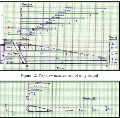
[image:24.612.154.539.288.666.2]

The FDTD method has an ability to deal with problems incorporating materials with geometrical in-homogeneities. With an arrangement of the fields in the Yee, the object will be constructed. This construction uses a combination of these simple object where it uses the term ‘brick’, which has its faces parallel to the Cartesian coordinates axes and can be represented by two corner point; [1] the point with lower x, y, and z coordinates and [2] the point with upper x, y, and z. Below, Figure 2 and 3 show the measured of wing and Table 2 represent a values Cartesian Coordinates Axes for lower and upper for each brick.

Figure 1.2: Top view measurement of wing-shaped