Spatial patterns of greenhouse gas emission in a tropical rainforest in
Indonesia
Shigehiro Ishizuka
1,*, Anas Iswandi
2, Yasuhiro Nakajima
3, Seiichiro Yonemura
3,
Shigeto Sudo
3, Haruo Tsuruta
3and Daniel Muriyarso
41Forestry and Forest Products Research Institute, Sapporo, Hokkaido 062-8516, Japan;2Department of Soil
Science, Bogor Agricultural University (IPB), Jl. Raya Pajajaran, Bogor 16143, Indonesia;3National Institute
for Agro-Environmental Sciences, Tsukuba, Ibaraki 305-8604, Japan;4Department of Geophysics and
Meteorology, Bogor Agricultural University (IPB), Jl. Raya Pajajaran, Bogor 16143, Indonesia; *Author for correspondence (tel.: +81-11-851-4131; fax: +81-11-851-4167; e-mail: [email protected])
Key words: Flux measurement, Geostatistics, Greenhouse gas, Semivariogram, Spatial variability, Sumatra of Indonesia
Abstract
Spatial patterns of CO2, CH4, and N2O flux were analyzed in the soil of a primary forest in Sumatra, Indonesia.
The fluxes were measured at 3-m intervals on a sampling grid of 8 rows by 10 columns, with fluxes found to be below the minimum detection level at 12 points for CH4and 29 points for N2O. All three gas fluxes distributed
log-normally. The means and standard deviations of CO2and CH4fluxes calculated by the maximum likelihood
method were 3.68 ⫾ 1.32 g C m–2 d–1 and 0.79 ⫾ 0.60 mg C m–2d–1, respectively. The mean and standard deviation of N2O fluxes using a maximum likelihood estimator for the censored data set was 2.99 ⫾ 3.26g N
m–2h–1. The spatial dependency of CH4fluxes was not detected in 3-m intervals, while weak spatial dependency
was observed in CO2and N2O fluxes. The coefficients of variation of CH4 and N2O were higher than that of
CO2. Some hot spots where high levels of CH4and N2O were generated in the studied field may increase the
variability of these gases. The resulting patterns of variability suggest that sampling distances of ⬎ 10 m and
⬎ 20 m are required to obtain statistically independent samples for CO2 and N2O flux in the studied field,
respectively. But because of weak or no spatial dependency of each flux, a sampling distance of more than 10 m intervals is enough to prevent a significant problem of autocorrelation for each flux measurement.
Introduction
CO2, CH4and N2O have been targeted as greenhouse
gases 共Prather et al. 2001兲. It is very important to know the precise variation in the intensity of these gas fluxes in tropical regions. Bouwman et al.共1993兲 es-timated the annual global N2O emission from soils as
6.8 Tg N, 80% of which was derived from the trop-ics. The global CH4 uptake rate by soils was
estimated as 15 to 35 Tg y–1, and humid tropical
for-est accounts for 10 to 20% of this共Potter et al. 1996兲. The annual CO2flux from soils to the atmosphere is
estimated to be 76.5 Pg C y–1 globally 共Raich and Potter 1995兲, and the CO2 flux from tropical moist
forest is the highest of all terrestrial ecosystems
共Raich and Potter 1995兲.
1995兲, soil infiltration rate 共Vieira et al. 1981兲, and enzyme activities共Bergstrom 1998兲in order to clarify spatial structure, and various review articles have been published共Parkin 1993; Goovaerts 1998兲. In the studies of greenhouse gas emissions, clarification of the spatial variability is one of the intensively studied categories, especially for N2O emissions. N2O
emis-sions are well known to show high spatial variability in various land-uses 共Velthof et al. 1996; Verchot et al. 1999兲and many reports have focused on the im-portance of the location on the slope for N2O
emis-sion and denitrification共Pennock et al. 1992; Reiners et al. 1998; Ishizuka et al. 2000兲. But there are few reports using geostatistical analysis in order to clarify the spatial structure for N2O emission 共Ambus and
Christensen 1994; Velthof et al. 1996; Clemens et al. 1999; Weitz et al. 1999兲. Probably because of the relatively smaller coefficient of variation of CO2flux
in the field, less attention has been paid to the spatial structure of CO2 flux. For this reason there is little
information about an adequate sampling distance for CO2to minimize autocorrelation共Ambus and
Chris-tensen 1994; Rayment and Jarvis 2000兲. This short-age of information on the spatial structure of CO2
fluxes is also applicable to that of CH4flux, especially
in tropical regions where CH4flux shows high
vari-ability 共Verchot et al. 2000兲 and information on the spatial structure may be more important.
Our objectives are to present preliminary informa-tion about the spatial structure of CO2, CH4and N2O
emissions in a 21 by 27 m area in a tropical rain for-est in Sumatra, Indonesia by geostatistical analysis and to contribute to the progress of the knowledge on the sampling design of these gas fluxes in such tropi-cal regions.
Material and methods
Sampling site and sampling design
To determine the spatial variation of greenhouse gas emissions from tropical rain forests in Indonesia, we conducted sampling on an 8 ⫻10 grid in a primary forest on 14 September 2001. The mean annual rain-fall was 2400 mm y–1 for 1998 through 2001. The mean soil temperature at the depth of 5 cm was 26 ºC in this experimental period. More detailed informa-tion on this forest has been described elsewhere
共Ishizuka et al. 2002兲as the same forest as the plot P1 and P2 in Pasir Mayang Research Site兲.
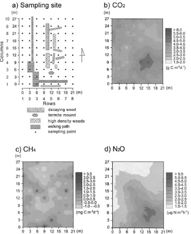
A sampling grid was prepared on the studied field, with 8 rows oriented E–W and 10 columns N–S共 Fig-ure 1兲. The interval between sampling points was 3 m. A set of 20 chambers was used for flux measure-ment. The gas samples for flux measurement were taken first from the westernmost two rows共1 and 2兲. After sampling from rows 1 and 2, we removed the chambers and set them on rows 3 and 4 and so on until all 80 points were sampled. The fluctuation of soil temperature did not affect the flux measurement in this experimental period, because it was relatively small 共the mean and standard deviation of soil tem-perature at 5 cm depth were 26.0 ⫾ 0.2 ºC and the difference between maximum and minimum temper-ature was 0.6 ºC兲. We took three time series共0, 10, 20 min兲 of gas samples per chamber 共0.25 m diam-eter, 0.15 m height兲after covering the chamber with a lid. The gas concentration was determined by two gas chromatographs 共Shimazu GC-9A-TCD-FID and Shimazu GC-14B-ECD兲. The methods of sampling transportation and gas analysis are detailed elsewhere
共Ishizuka et al. 2005共this issue兲兲.
Statistical analysis
For each flux measurement we calculated the mini-mum significant flux 共␣⫽0.10; Hutchinson and Liv-ingston 1993兲. All flux was significant from zero in the CO2flux calculation. The minimum fluxes
con-sidered as significant from zero for CH4 and N2O
were 0.18 mg C m–2d–1and 1.49g N m–2h–1, re-spectively, and we defined the trace data as the flux whose absolute value was below these values. For the CH4 flux, because the trace data 共n⫽12兲 were
supposed to be distributed evenly between ⫺0.18 and 0.18 mg C m–2 d–1and the bias to replace them
to zero could be considered negligible for further cal-culation, the trace data were replaced as zero. For the trace data of N2O flux, we used two ways for further
calculation. One is the calculation of arithmetic mean and standard deviation and geostatistical analysis, in which the trace data were replaced with one half of the detection limit 共namely, 0.75 g N m–2 h–1兲 共Kushner 1976; Gilbert 1987兲. And the other is the estimation of log-transformed mean and standard de-viation of the flux, using the maximum likelihood method for the censored data set共Gilbert 1987; Kut-tatharmmakul et al. 2000兲.
CO2and CH4obtained in this study was log-normal,
we adopted the maximum likelihood method共Parkin et al. 1988兲of estimating the mean and coefficient of variation for these gases, in the light of the relatively low skewness of data and sufficiency of data points.
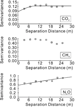
Experimental variograms were used to quantify the spatial dependence of CO2, CH4 and N2O fluxes
共GS⫹version 5.3b, Gamma Design Software, Michi-gan, USA兲. According to the log-normal frequency distributions in these fluxes, flux data for them were log-transformed for geostatistical analysis.
Figure 1.The sampling design and properties of the sampling site共a兲, and the maps of共b兲CO2,共c兲CH4, and共d兲N2O fluxes within the study
area. The maps of CO2and CH4were created by the inverse distance weighting method. The map of N2O was created by block kriging with
To analyze the relationship between each of the gas fluxes, we used nonparametric statistics of Spearman rank correlation.
Results and discussion
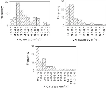
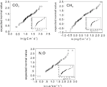
The results of each flux are summarized in Table 1. All three gas fluxes were log-normally distributed
共Figure 2兲, as indicated by a Q-Q plot of log-trans-formed and non-translog-trans-formed fluxes共Figure 3兲. How-ever, at 12 points of CH4flux and 29 points of N2O
flux 共15 and 36% of all sampling points, respec-tively兲, the flux was under the detection limit 共Table 1兲. The log-normal distribution of N2O flux contrasts
with the results of other reports, suggesting a normal distribution共Clemens et al. 1999兲, but agrees with the results of still other reports 共e.g., Ambus and
Chris-Table 1.The statistical data of CO2, CH4and N2O emission rates.
Number of observa-tions of trace data
Untransformed Maximum Likelihood by
Log-transformed Data
Mean Median SD Min. Max. Skewness CV共%兲 Mean SD CV共%兲
共g C m–2d–1兲 共g C m–2d–1兲
CO2 0 3.68 3.26 1.32 1.56 7.18 0.79 36 3.68 1.32 36
共mg C m–2d–1兲 共mg C m–2d–1兲
CH4 12 0.83
a 0a 2.18a ⫺1.34 8.28 1.63a 136a 0.80a 0.61a 76a
共g N m–2h–1兲 共
g N m–2h–1兲
N2O 29 2.84
b 1.98b 2.60b Tr.c 11.0b 1.53b 92b 2.99d 3.26d 109d
aThe trace data were replaced as 0;bThe trace data were replaced as one half of the detection limit;cTrace;dUsing maximum likelihood
estimation from the censored data sets共Gilbert 1987兲.
Figure 2.Frequency distribution of CO2共upper left兲, CH4共upper right兲, and N2O共lower兲fluxes.
tensen 1994兲. The means and standard deviations of CO2and CH4flux calculated by the maximum
like-lihood method were 3.68 ⫾1.32 g C m–2 d–1 and 0.79 ⫾0.60 mg C m–2 d–1, respectively. The mean and standard deviation of N2O was 2.99 ⫾ 3.26g
N m–2h–1by the estimation of log-transformed mean and standard deviation of the flux, using the maximum likelihood method for a censored data set. The coefficient of variation for log-transformed val-ues of CH4共76%兲and N2O共109%兲was higher than
that for CO2共36%兲 共Table 1兲. Between CO2and CH4
flux and between CO2and N2O flux there was a weak
positive correlation 共Spearman rank correlation,
R⫽0.345 and 0.354, respectively; Table 2兲.
The variograms of log-transformed CO2 flux
showed weak spatial dependence 共Figure 4兲, and a spherical model was selected according to the mini-mum residual sums of squares 共RSS; 2.026E⫺04,
R2⫽0.623兲. Few studies have addressed the spatial variability of soil CO2 efflux 共Rayment and Jarvis
2000兲. The value of the range parameter in this study is relatively greater than in Rayment and Jarvis
共2000兲. The range parameter is 10 m, indicating that
to obtain statistically independent samples for CO2
flux we need a sampling interval of greater than 10 m.
The semivariance of N2O gradually increased with
the increase of the separation distance共Figure 4兲, fit-ted by an exponential model with the parameters of sill, range and nugget as 1.62, 195 m and 0.55, re-spectively共R2⫽0.842; RSS⫽1.97兲. This pattern of semivariogram was comparable with a previous report of analysis of N2O fluxes in mown and grazed
grassland共Velthof et al. 1996兲. The range and sill ob-tained are not precisely determined, because we did not make measurements at distances of more than 27 m. The nugget is equivalent to 1.73 g N m–2 h–1,
which is close to the detection limit共1.49g N m–2 h–1兲, this result suggesting that the nugget effect is mainly due to measurement error. The range param-eter of 195 m is unreliable as mentioned above, but the result suggests that to obtain statistically indepen-dent samples for N2O flux we need a sampling
inter-val of greater than 20 m in this site.
The variograms of log-transformed CH4flux show
no change of semivariance with distance 共Figure 4兲,
Figure 3.Q-Q plot of log-transformed fluxes: CO2共upper left兲, CH4共upper right兲, and N2O共lower兲fluxes. The inset is a Q-Q plot of
indicating that there is no spatial dependence for CH4
flux over 3-m intervals. The 3-m intervals of grid are too large and the distance showing spatial depen-dency may be smaller than 3 m. Previous studies suggest that there are ‘hot spots’ where high levels of N2O are generated共e.g., Kessel et al. 1993兲. We also
observed relatively high N2O or CH4flux at several
points, and the spatial dependence was considered low due to these hot spots.
According to our measurements, for both CH4and
N2O emissions, the evaluation of total fluxes is
sig-nificantly affected by hot spot coverage by the cham-bers. This hot spot heterogeneity could be greater than the effect of nearby autocorrelation. Because of weak or no spatial dependency of each flux, the sampling
distance in more than 10 m intervals is enough to prevent a significant problem of autocorrelation for each flux measurement.
Using the parameter from variogram analysis, a map of N2O flux was produced by block kriging
共Figure 1兲 and the maps of CO2and CH4were
pro-duced by the inverse distance weighting method. The greatest CO2 flux concentrated around an area with
dense weed共near the point of row 5 to 6, column 4, in Figure 1兲, suggesting that root respiration of weed is an important source in the studied field. The sam-pling points that showed high CH4flux共⬎1.8 mg C
m–2d–1兲were mainly located along the walking path
共Figure 6兲. The plausible sources for this high CH4
flux were termites. In this forest the termite popula-tion can be high 共Ishizuka et al. 2005 共this issue兲兲. Also it is possible that the soil along the walking path was compacted by human activity and its soil gas diffusivity was reduced, limiting the diffusion of oxy-gen to the deeper soil. As a result of high CH4
pro-duction by anaerobic methanogenesis, propro-duction exceeded consumption. Our data do not indicate which idea is more favorable. Further research is needed to clarify the source of CH4. These results
suggest that the spatial patterns of these greenhouse gases are strongly affected by human foot traffic through the site, plants and insects.
Trace gas flux measurements were made only one time. The spatial dependency may fluctuate with the fluctuation of soil properties. Velthof et al. 共1996兲
suggested that the strong temporal variation of flux controlling factors may affect the stability of semivar-iograms of fluxes, and generally applicable semivari-ograms cannot be obtained. The sampling period in this research was mid-September, which is the transi-tional period from dry to wet season. Averaged soil water content in September was 0.11 Mg m–3, which
is relatively dry but close to the annual mean of soil water content 共0.13 ⫾ 0.03 Mg m–3兲 in this forest
共non-calibrated values, measured by TDR at 7.5 cm depth for two years, unpublished data兲. It is possible that drastic change of spatial variation could occur after heavy rainfall. We expect, however, that the general picture provided in this spatial study is typi-cal of the site in which the spatial variation of CO2
flux is smaller than those of CH4and N2O. There is
little information about the spatial structure of green-house gas emissions in tropical forests and additional studies are needed to produce more general images.
Figure 4.Variograms of log-transformed fluxes of CO2共top兲, CH4 共middle兲, and N2O共bottom兲. The line in the variograms of CO2flux
was fitted by a spherical model; the sill, range and nugget are 0.123, 10.0, and 0.083, respectively. The line in the variograms of N2O flux was fitted by an exponential model; the sill, range and
nugget are 1.62, 195 m and 0.55, respectively.
Table 2.Non-parametric correlation coefficient of all gas fluxes.
Acknowledgements
This study was managed under the project ‘The im-pact of land-use/cover change in terrestrial ecosys-tems of tropical Asia on greenhouse gas emissions’ in the Global Environmental Research Program sup-ported by a grant from the Ministry of the Environ-ment, Japan. We thank Mr. Zuhdi and Mr. Ermadani of Jambi University for their assistance in fieldwork. We also thank the staff at Pasir Mayang Research Site. We extend our thanks to the assistants Ms. Ban-zawa, Ms. YoshiBan-zawa, Ms. Matsuoka at NIAES, and Ms. Takeuchi at FFPRI.
References
Ambus P. and Christensen S. 1994. Measurement of N2O emission
from a fertilized grassland: An analysis of spatial variability. J. Geophys. Res. 99: 16549–16555.
Bergstrom D.W., Monreal C.M., Millette J.A. and King D.J. 1998. Spatial dependence of soil enzyme activities along a slope. Soil Sci. Soc. Am. J. 62: 1302–1308.
Bouwman A.F., Fung I., Matthews E. and John J. 1993. Global analysis of the potential for N2O production in natural soils.
Global Biogeochem. Cycles 7: 557–597.
Clemens J., Schillinger M.P., Goldbach H. and Huwe B. 1999. Spatial variability of N2O emissions and soil parameters of an
arable silt loam – a field study. Biol. Fertil. Soils 28: 403–406. Gilbert R.O. 1987. Estimating the mean and variance from censored data sets. In: Statistical Methods for Environmental Pollution Monitoring. John Wiley and Sons, New York, USA, pp. 177–185.
Goovaerts P. 1998. Geostatistical tools for characterizing the spa-tial variability of microbiological and physico-chemical soil properties. Biol. Fertil. Soils 27: 315–334.
Gourbiere F. and Debouzie D. 1995. Spatial distribution and esti-mation of forest floor components in a 37-year-oldCasuarina equisetifolia 共Forst.兲 plantation in coastal Senegal. Soil Biol. Biochem. 27: 297–304.
Hutchinson G.L. and Livingston G.P. 1993. Use of chamber sys-tems to measure trace gas fluxes. In Harper L.A.共ed.兲, Agricul-tural Ecosystem Effects on Trace Gases and Global Climate. American Society of Agronomy, Madison, Wisconsin, USA, pp. 63–78.
Ishizuka S., Iswandi A., Nakajima Y., Yonemura S., Sudo S., Tsu-ruta H. and Murdiyarso D. 2005. The variation of greenhouse gas emissions from soils of various land-use/cover types in Jambi province, Indonesia. Nutr. Cycling Agroecosyst. 71: 17–32共this issue兲.
Ishizuka S., Tsuruta H. and Murdiyarso D. 2002. An intensive field study on CO2, CH4and N2O emissions and soil properties at four
land-use types in Sumatra, Indonesia. Global Biogeochem. Cycles 16: 1049 doi:10.1029/2001GB001614.
Ishizuka S., Sakata T., Tanikawa T. and Ishizuka K. 2000. N2O
emission and spatial distribution in a Japanese deciduous forest. J. Jpn. For. Soc. 82: 62–71.
Kessel C., Pennock D.J. and Farrell R.E. 1993. Seasonal variations in denitrification and nitrous oxide evolution at the landscape scale. Soil Sci. Soc. Am. J. 57: 988–995.
Kushner E.J. 1976. On determining the statistical parameters for pollution concentration from a truncated data set. Atmos. Envi-ron. 10: 975–979.
Kuttatharmmakul S., Smeyers-Verbeke J., Massart D.L., Coomans D. and Noack S. 2000. The mean and standard deviation of data, some of which are below the detection limit: an introduction to maximum likelihood estimation. Trends Anal. Chem. 19: 215– 222.
Oliver M.A. and Webster R. 1991. How geostatistics can help you. Soil Use Manage. 7: 206–217.
Parkin T.B. 1993. Spatial variability of microbial processes in soil – a review. J. Environ. Qual. 22: 409–417.
Parkin T.B., Meisinger J.J., Chester S.T., Starr J.L. and Robinson J.A. 1988. Evaluation of statistical estimation methods for log-normally distributed variables. Soil Sci. Soc. Am. J. 52: 323–329.
Paz-González A. and Taboada M.T. 2000. Nutrient variability from point sampling on 2 meter grid in cultivated and adjacent forest land. Commun. Soil Sci. Plant Anal. 31: 2135–2146.
Pennock D.J., van Kessel C., Farrell R.E. and Sutherland R.A. 1992. Landscape-scale variations in denitrification. Soil Sci. Soc. Am. J. 56: 770–776.
Potter C.S., Davidson E.A. and Verchot L.V. 1996. Estimation of global biogeochemical controls and seasonality in soil methane consumption. Chemosphere 32: 2219–2246.
Prather M., Ehhalt D., Dentener F., Derwent R., Dlugokencky E., Holland E. et al. 2001. Athmospheric chemistry and greenhouse gases. In: Houghton J.T., Ding Y., Griggs D.J., Noguer M. van der Linden P.J., Dai X. et al.共eds兲, Climate Change 2001: The Scientific Basis. Contribution of Working Group I to the Third Assessment Report of the Intergovernmental Panel on Climate Change. Cambridge University Press, Cambridge, UK and New York, USA, pp. 239–287.
Raich J.W. and Potter C.S. 1995. Global patterns of carbon dioxide emissions from soils. Global Biogeochem. Cycles 9: 23–36. Rayment P.G. and Jarvis P.G. 2000. Temporal and spatial variation
of soil CO2efflux in a Canadian boreal forest. Soil Biol.
Bio-chem. 32: 35–45.
Reiners W.A., Keller M. and Gerow K.G. 1998. Estimating rainy season nitrous oxide and methane fluxes across forest and pas-ture landscapes in Costa Rica. Water Air Soil Pollut. 105: 117– 130.
Velthof G.L., Jarvis S.C., Stein A., Allen A.G. and Oenema O. 1996. Spatial variability of nitrous oxide fluxes in mown and grazed grasslands on a poorly drained clay soil. Soil Biol. Bio-chem. 28: 1215–1225.
Verchot L.V., Davidson E.A., Cattânio J.H., Ackerman I.L., Erick-son H.E. and Keller M. 1999. Land use change and biogeochem-ical controls of nitrogen oxide emissions from soils in eastern Amazonia. Global Biogeochem. Cycles 13: 31–46.
Verchot L.V., Davidson E.A., Cattânio J.H. and Ackerman I.L. 2000. Land-use change and biogeochemical controls of methane fluxes in soils of eastern Amazonia. Ecosystems 3: 41–56. Vieira S.R., Nielsen D.R. and Biggar J.W. 1981. Spatial variability
Weitz A.M., Keller M., Linder E. and Crill P.M. 1999. Spatial and temporal variability of nitrogen oxide and methane fluxes from a fertilized tree plantation in Costa Rica. J. Geophys. Res. 104: 30097–30107.
Yost R. S., Uehara G. and Fox R. L. 1982. Geostatistical analysis of soil chemical properties of large land areas. I. Semi-variograms. Soil. Sci. Soc. Am. J. 46: 1028–1032.