DOI: 10.12928/TELKOMNIKA.v14i3A.4400 237
Time-frequency Analysis of Track Irregularity Based on
Orthogonal Empirical Mode Decomposition
Ling Zhao*1, Darong Huang2, Honggang Wang3, Hongtao Yu4, Xiaoyan Chu5
1,2,3,5
School of Computer Science and Technology, Chongqing Jiaotong University, Chongqing,400074, China
1
School of Automation, Chongqing University, Chongqing, 400030, China
4Department of Mechanical Engineering, Texas A&M University, College Station, 77840, United States
*Corresponding author, e-mail:[email protected]
Abstract
A method of extracting transient features of a non-stationary signal was proposed based on the combination of orthogonal empirical mode decomposition (OEMD) and the Hilbert transform. After obtaining orthogonal intrinsic mode functions, the instantaneous frequency and amplitude can be calculated, so problems existing in the original Hilbert-Huang Transform (HHT) method, such as mode aliasing, can be solved. The track irregularity signal is studied with the OEMD method, and the statistical and analytic result indicates that there are relatively serious short wave and long wave track irregularities in the sample signal. Analysis of track irregularities using OEMD is a new technical method for guaranteeing the safe running of railway.
Keywords: track irregularity, orthogonal empirical mode decomposition, Hilbert transform, time-frequency analysis
Copyright © 2016 Universitas Ahmad Dahlan. All rights reserved.
1. Introduction
The complex coupled motion between wheel and rail is the result of the combined effects of the vehicle, rail and external environment; this combination of factors determines the complexity and multi-factorial nature of its vibration signals. However, nonlinear changes, such as the geometry and suspension stiffness of the wheel and rail as they are in contact, turn the coupled vibration between vehicle and track into a nonlinear and non-stationary stochastic process [1]. The track irregularity is the foremost excitation source of vehicle vibration, and it magnifies the dynamic effects of the train combining with the rapid increase of the train speed; this can directly affect not only the safety and smoothness of the train, but it can also accelerate the development of the track irregularity condition. Therefore, it is a significant topic that should be part of a thorough study about driving safety and comfort [2].
Currently, the methods for analyzing test data, such as the method based on Fourier transform and the method based on the wavelet analysis [3, 4], are generally carried out within the time domain, frequency domain and amplitude domain. The Fourier method is applicable to the linear and stable signals, achieving good analytic results. However, the Fourier transforms use multiple sources of input to produce an average result, and the information extraction for this type of problem can only be conducted from a single perspective within the overall properties of time domain, frequency domain and amplitude domain. The result is that the varying characteristics of non-stationary signals cannot be reflected by Fourier transform; moreover, these varying characteristics also affect the application of the method in the field of the analysis for the non-stationary signals. The wavelet analysis can reflect the features of the time domain and the characteristics of the frequency domain for vibration signals at the same time. The wavelet analysis can also realize the time-frequency characteristic utilizing the inner product of the mother wavelet and the signal. But because the result of localization analysis is based on the mother wavelet sketching and parallel moving, the analysis result relies on the choice of wavelet to a large extent, and the adaptability is not ideal. In addition, the aliasing existing in a wavelet transform will affect the accuracy of the signal analysis.
Moreover, when aiming at the nonlinear and non-stationary signals, this method can make an adaptive analysis, and its advantages in many fields are on the horizon. Two parts, the empirical mode decomposition (EMD) and the Hilbert transform, are contained in the Hilbert-Huang transform (HHT). EMD is the core part of the HHT; it is the part that realizes the linearization and steady process for the nonlinear and non-stationary data. The intrinsic mode function (IMF) is proposed in HHT, which guarantees that the instantaneous frequency and the instantaneous amplitude-obtained by Hilbert transform for each component-have reasonable physical meaning, and thus realizing the correct time-frequency analysis. During the screening process of the intrinsic mode function, cubic spline function, which constitutes the upper envelope and the lower envelope, will emerge divergent on both sides of the data sequence. Moreover, with a continuous selection process, the divergent results will inwardly pollute the entire sequence gradually, distorting the obtained results; we call this question the end effect.
Now many new methods, such as the mirroring closed continuation method, the continuation method based on neural networks, the continuation method based on support vector machines, the waveform feature matching the continuation method, the mask signal method and so on, are put forward by many scholars at home and abroad to solve the problem of the end effect; however, limitations still exist for each method exist [6]. The orthogonal empirical mode decomposition (OEMD) based on band-pass filtering is proposed in this paper, and the method has strict orthogonality and completeness, solving the issues of modal aliasing and false modals caused by the end effects. The signal is decomposed into the various IMFs and the residual function by means of OEMD, and then the Hilbert transform is conducted for each IMF to seek instantaneous frequency and instantaneous amplitude; this procedure detects the information about the time-frequency domain for the mutations and various components of the non-stationary signals. The method is applied to the analysis of a track irregularity signal.
2. Orthogonal Empirical Mode Decomposition
Essentially, empirical mode decomposition means that the non-stationary signals are treated by an axisymmetric method, which separates the intrinsic mode functions according to their frequency in descending order. The intrinsic mode functions need to satisfy these two conditions: 1) the number of extreme points equals the number of zero-crossing points, or their difference is one; 2) the mean value of the envelope which is constituted by the maximum and the minimum values of the dates equals zero for any point.
It is difficult to meet the second condition mentioned above, so various criteria are proposed by different researchers to achieve ideal results. Aiming at the second condition, the following criteria are proposed: the ratio of the signals’ local mean curve and the energy of the signal is smaller than a given threshold; this threshold is determined by the characteristics of the components contained in the signals and the decomposition accuracy of the signals.
Generally, the signals need to filter the IMF using EMD. In fact, the Empirical Mode Decomposition is a process of adaptive filtering; it obtains the intrinsic mode functions using an adaptive band-pass filter [7], and the specific decomposition process is shown as below:
First, let signal to be detected be x(t), and its frequency range is
0,fc
. Then, the frequencyf
1 can be found by searching within the frequency range above, makingx
(
t
)
pass through the ideal band-pass filter, and the filter is shown as below:
else f f f f
H1 1 c
0 1 )
( (1)
And then x(t) can meet the definition of IMF. Obtain the first IMF, and let it be c1(t).
Second, the frequency f2 is searched within
0,f1 to obtain the second IMF; that is to say the) (
2 t
c . The frequency f3 can be detected within
0,f2
to achieve c3(t). Then, the IMFs) ( , ), ( ),
( 2
1 t c t c t
c n and the residual function r(t) can be obtained by repeating the operation
above, and the decomposition process ends when fn 0 or r(t) is a monotonic function, or the
else f f f
Hd c
0 0 1 )
(
(2)
Let fn 0, and then the r(t)0. In order to find the frequency-modulated (FM) signals and amplitude-modulated (AM) signals, Hi(f) should be the filter with the most broadband.
It can be seen that when obtaining the k-th intrinsic mode function ck(t), the band-pass
filter used can be presented as below:
else f f f f
Hk k k-1
0 1 )
( (3)
When k1,f0 fc, let Ck(f)Hk(f)X(f), where X(f)FT
x(t) , and FT denotesthe Fourier transform, and Hk(f) represents the k-th filter. And then the k-th IMF
c
k(
t
)
can beexpressed asIFT
Ck(f)
; that is to say, ck(t)IFT
Ck(f)
, where IFT indicates the inverseFourier transform.
For any two intrinsic modes’ function components cj(t) and ck(t), according to the
Parseval's theorem, we can get the following formulation:
* * *
( ) ( )
( )
( )
( )
( )
( )
j k i ki k k
c t c t dt
C f C
f df
H f H
f C
f df
(4)
Where,
j
k
,f
j
f
k1, soH
j(
f
)
H
k(
f
)
0
, and then we can obtain the following formula successfully:*
( )
( )
0
j k
c t c t dt
(5)Obviously, any two components
c
j(
t
)
andc
k(
t
)
are mutually orthogonal and onecomponent has nothing to do with the other; moreover, the conversion does not affect the represented function itself. Similarly, we can demonstrate that
r
(
t
)
is orthogonal to anyc
k(
t
)
.1 1
( ) ( ) ( ) ( ) ( ) ( ) ( )
n n
i i d
i i
c f R f H f X f H f X f X f
(6)So 1
( )
( )
( )
n i ix t
c t
r t
(7)It can be seen from the decomposition process above that every IMF can be found by applying orthogonal empirical mode decomposition to the signal; meanwhile, IMF is the result that can be obtained by filtering the original signal. Therefore, the end effect problem is not too serious, and the previous components’ boundary effects will not affect the components obtained afterward. The phenomenon of divergence and inward pollution, which appear in the data at both ends when general EMD is adopted, will not happen with the method we propose, which overcomes the end effect problem that exists in EMD [8, 9].
3. Hilbert Transform
First, the signal is decomposed into several IMFs and residual function by means of OEMD; second, the instantaneous frequency and the instantaneous amplitude are calculated for every IMF using the Hilbert transform.
)
(
t
v
can be achieved by applying the Hilbert transform to the signalu
(
t
)
, andv
(
t
)
can be shown as below:1
( )
( )
u
v t
d
t
(8)
Then, the analytical signal is constructed as follows:
( )
( )
( )
( )
( )
ji ti i
z t
u t
jv t
a t e
(9)Thus, the amplitude function and phase function are all obtained and can be expressed by the following formulas (6) and (7) respectively:
2 2
( )
( )
( )
i i i
a t
u t
v t
(10)
( )
( )
arctan
( )
i i
i
v t
t
u t
(11)At the same time, the instantaneous frequency can be obtained as below:
( )
1
1
( )
( )
.
2
2
i
i i
d
t
f t
t
dt
(12)Therefore, the instantaneous frequency and amplitude are used to depict the frequency of the signal instead of the power spectrum. So, the Hilbert spectrum can be denoted as below:
( )
1
( , )
Re
( )
in
j t dt i
i
H
t
a t e
(13)
where Re means that the real part is adopted, and the residual component ri(t) is
ignored.
However, the Hilbert marginal spectrum
h
(
)
can be expressed as follows:0
( )
T( , )
where T indicates the total length of the signal. With time and frequency conversion,
) ,
( t
H can describe the signals’ conversion law over the entire frequency range. The instantaneous amplitude and instantaneous frequency are the variables of time, constituting the three-dimensional spectrum of time, frequency and amplitude, i.e., the Hilbert spectrum. However, with the frequency conversion, h() reflects the signals’ transformational situation over the entire frequency range.
4. Results and Analysis
[image:5.595.195.408.252.337.2]The detection signals of track irregularity are obtained from the comprehensive test train data of the trunk railway from the downstream direction in 2012; the sampling point is 4000/km. The signals’ time-domain waveform can be presented as Figure 1.
[image:5.595.206.392.382.532.2]Figure 1. The sampling signals’ time-domain waveform
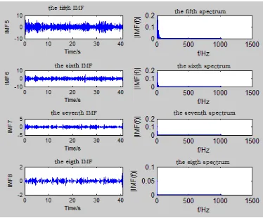
Figure 2. The first four IMFs and their spectra
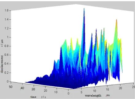
[image:5.595.204.391.577.732.2]The sampling signals are processed by means of orthogonal empirical mode decomposition, and the first eight decomposition results are shown in Figure 2 and Figure 3, which contain all of the frequency components. Then, the Hilbert Transform is applied to the signals to achieve the Hilbert spectrum, shown in Figure 4.
Figure 4. The Hilbert spectrum
For the signals of the track irregularity, the amplitude is relatively large at the point of 13 meters, and also at or near the point of 25 meters, of the wavelength; this illustrates that the irregularity is generated by the periodic irregularity of subsidence of bed railway tunnel road in the track rail joint or welded joint. However, the existence of the wavelength within the range from 15.8 meters to 30 meters indicates the presence of adverse track disease in this track direction; this further indicates that a check should be carried out for distances of 250 meters, 482 meters, 1333 meters, 1661 meters and so on. The test results show that the long-wave irregularity is the main band of track disease for the sample segment. At increasing levels of speed, the long-wave irregularity will significantly affect the driving safety and comfort of the train. Railway works departments should strengthen the maintenance of the long-wave track.
5. Conclusion
Aiming at the problems existing in EMD, a novel HHT method is proposed based on the OMED and the Hilbert transform, and the method is applied to the feature information extraction of railway track irregularities. In doing so, we reach the following conclusions from the experimental results.
(1)Inheriting the advantages of the adaptive multi-resolution of the HHT, the method proposed in this paper realizes the signals’ orthogonal decomposition and overcomes the modal aliasing. In addition, our method does not need to make pretreatment.
(2)Through time-frequency analysis of the track irregularities, we find that different levels of shortwave and long-wave irregularity are both present in the sample track irregularities. This will be an argument for the railway works departments to master the amplitude and wavelength distribution of track irregularities. If they do so, track irregularities can be maintained and repairs carefully targeted; this will have certain significance in the field of engineering applications.
Acknowledgements
References
[1] Ning YZ, Zhou XL, Xu QY. Analysis of track irregularity and car-body vibration response on wavelet transform. Journal of Railway Science and Engineering. 2013; (3): 28-33.
[2] Ning J, Zhu CQ, Zhang B. An approach for signal analysis of track irregularity based on EMD and Cohen's Kernel. Journal of Vibration and Shock. 2013; 32(4): 31-37.
[3] Dadkhah M, Sutikno T. Phishing or Hijacking? Forgers Hijacked DU Journal by Copying Content of Another Authenticate Journal. Indonesian Journal of Electrical Engineering and Informatics (IJEEI). 2015; 3(3): 119-120.
[4] Wang J. Robust Pitch Detection Based on Recurrence Analysis and Empirical Mode Decomposition. TELKOMNIKA Indonesian Journal of Electrical Engineering. 2015; 14(1): 116-122.
[5] Dadkhah M, Obeidat MM, Jazi MD, Sutikno T, Riyadi MA. How can we identify hijacked journals?. Bulletin of Electrical Engineering and Informatics. 2015; 4(2): 83-87.
[6] Li ZW, Lian SL, Zhou JL. Time-frequency Analysis of Track Irregularity Based on Improved Empirical Mode Decomposition Method. Journal of Tongji University (Natural Science). 2012; (5): 702-707. [7] LI ZW, Lian SL. Analysis of track irregularity signal by improved Hilbert-Huang Transform. Journal of
Shenzhen University Science and Engineering. 2012; (3): 270-275.
[8] Makwana NH, Makwana N, Mishra N, Sagar B. Hilbert Transform Based Adaptive ECG R-Peak Detection Technique. International Journal of Electrical and Computer Engineering. 2012; 2(5): 639-643