http://dx.doi.org/10.12988/ams.2014.43189
Hybrid Empirical Mode Decomposition-ARIMA
for Forecasting Price of Rice
Sarah Abadan and Ani Shabri
Department of Mathematical Sciences, Faculty of Science Universiti Teknologi Malaysia, 81310 Skudai, Johor, Malaysia
Copyright © 2014 Sarah Abadan and Ani Shabri. This is an open access article distributed under the Creative Commons Attribution License, which permits unrestricted use, distribution, and reproduction in any medium, provided the original work is properly cited.
Abstract
The prices of rice keep changing from time to time. It creates risks to producers, suppliers, consumers, and other parties that involved in marketing and production of rice. Thus, it is important to do forecasting on rice prices data set. This paper tries to apply a hybrid methodology which is an integration of empirical mode decomposition (EMD) and autoregressive integrated moving average (ARIMA). The EMD-ARIMA is applied on the data of the monthly prices of rice in Malaysian Ringgit (MYR) per metric ton. Forecasting result found that EMD can improve the accuracy of the ARIMA forecasting on the prices of rice based on the comparison of root mean squared error (RMSE) and mean absolute error (MAE).
Keywords: ARIMA, EMD-ARIMA, rice prices, forecasting
1 Introduction
From time to time, the prices of rice are changing and volatile. The instability of rice prices creates significant risks to producers, suppliers, consumers, and other parties that are involved in the marketing and production of rice. In risky conditions and amidst price instability, forecasting is very helpful in making decisions. Accurate price forecasts are certainly important to alleviate efficient decision making as there is time lag intervenes between making decisions and the actual output of the commodity in the market [1].
2 Literature reviews
The prices of rice data has been forecasted by many of previous researchers with various types of methods. Sandika [8] applied growth models on three types of rice in Sri Lanka which are samba, kakulu, and nadu. While Hassan et. al. [4] also applied growth models but on coarse rice prices in Bangladesh. However, the forecasting accuracy contributed by growth models do not as good as provided by stochastic time series model, which is ARIMA, but they do provide a simpler acceptable forecasting result [4]. The seasonal ARIMA (SARIMA) has been used by Tuong [9] on the high quality rice data in Vietnam. While in Iran, triple exponential smoothing (TES) and SARIMA are applied on forecasting the monthly price of Privileged Sadri rice in Guilan province and the result found out that SARIMA gives a better result [7].
ARIMA method is one of the most widely used by the previous researchers not only on the price of rice, but also on commodities prices as well. For examples, Hakan et. al. [3] used SARIMA in forecasting the tomato prices in Turkey, while Assis et. al. [1] used ARIMA and others methods to forecast the cocoa beans prices.
However, Xu et. al. [11] applied a hybrid forecasting method which is an integration of empirical mode decomposition (EMD) and ARIMA on a data set of commodities demand after natural disaster in China. As a result, EMD can improve the prediction accuracy of classical ARIMA forecasting method. EMD, which proposed by Huang et. al. [5], has been combined by previous researchers with other methods too to improve the result of that single method. For example, Wei et. al. [10] combined EMD and back-propagation neural networks (BPN) to predict the short-term passenger flow in metro systems, while Liu et. al. [6] used the hybrid of EMD and artificial neural networks to predict the wind speed.
3 Methodology
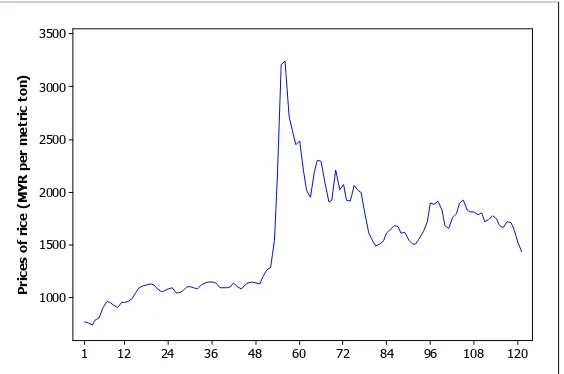
The data set involved in this analysis is the monthly prices of rice (MYR per metric ton) from October 2003 to October 2013. The data is collected from www.indexmundi.com. The figure 1 below shows the plot of the data set involved in this paper.
Figure 1: Graph of the prices of rice (MYR per metric ton)
From figure 1, we can see that the data fluctuated in non-seasonal and non-stationary pattern. According to Xu et. al. [11], EMD is a process method generally for nonlinear and non-stationary data set. Thus, this paper attempts to apply a hybrid methodology which is an integration of ARIMA and EMD to forecast the price of rice.
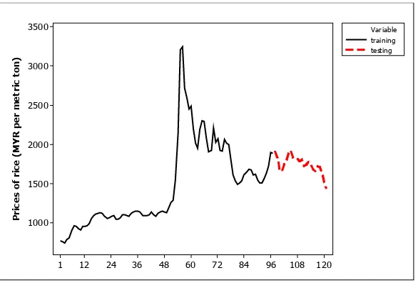
Figure 2: Graph of the training and testing set
3.1 ARIMA
ARIMA represents an autoregressive integrated moving average and introduced by Box and Jenkins [2]. ARIMA models are, in theory, the most general class of models for forecasting a time series which can be stationarized by transformations such as differencing, where the order of , , is classified as below
1. is the number of autoregressive terms 2. is the number of non-seasonal differences
3. is the number of lagged forecast errors in the prediction equation
Given a time series of the actual value, where is the time period, then ARIMA , , process is given by
⋯ ⋯
(1)
Where is a constant, , , … , are parameters of autoregressive (AR), , , … , are parameters of moving average (MA). The random errors, , are assumed to be independently and identically distributed with a mean of zero and constant variance of .
A stationary time series is one whose properties do not depend on the time at which the series is observed. More precisely, if is a stationary time series, then for all , the distribution of , … , does not depend on . Stationarity can be obtained by differencing the data set. The first difference is defined as
′ (2)
While the second difference is defined as
" 2 (3)
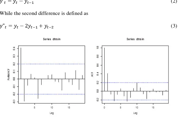
Figure 3: Partial autocorrelation function (PACF) and ACF of the training set
The order of and are determined with aid of the PACF and the ACF as shown in figure 3. All the possible models are listed for diagnostic checking with Ljung-Box test. The Ljung-Box test can be defined as
"#: The data are independently distributed " : The data are not independently distributed
The test statistic is
$ % % 2 ∑ '()*
+ ,
-,. (4)
Where % is the sample size, /0, is the sample autocorrelation at lag 1, and 2 is the number of lags being tested. For significance level 3, the critical region for rejection of the hypothesis of randomness is
Where 5 6,- is the α-quantile of the chi-squared distribution with 2 degrees of
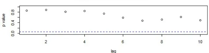
freedom. A good model, as shown in figure 4, has all large -values for the Ljung-Box statistics. It indicates that the residuals are patternless which explain that all the information has been extracted.
Figure 4: Graph of -values for Ljung-Box statistic
Next, Akaike information criterion (AIC) is used for model selection.
AIC 2 ln likelihood 2? (6)
Where likelihood is the probability of the data given a model and ? is the number of free parameters in the model. Generally, the model with the smallest value of AIC is chosen as the best model.
Last but not least, the selected model is used to forecast the testing data set. Then, the root mean squared error (RMSE) and mean absolute error (MAE) for both training and testing data set are taken, as shown in table 1, for comparing the accuracy with other method.
3.2 Empirical Mode Decomposition
The basic idea of EMD is to decompose time series into a sum of oscillatory functions which is called intrinsic mode functions (IMF). Each IMF must satisfy two conditions [5] which are:
1. In the whole data set, the number of extrema (maximum and minimum) and the number of zero-crossings must either equal or differ at most by one; 2. At any point, the mean value of the envelope defined by the local maxima
and the envelope defined by the local minima is zero.
The IMFs can be extracted from the time series data set through an iterative decomposition process as described as the following steps:
Step 1: Identify all the local extrema of time series ;
@AD+ ;
Step 3: Calculate the mean of the upper and lower envelops and let it as E ,
E @ABC @AD+ /2 (7)
Step 4: Extract the mean from the data and define the difference as ,
E (8)
Step 5: Check : if it satisfies those two conditions of IMF, output it as the Gth IMF and replace with the residue
H (9)
if is not an IMF, replace with .
Step 6: Repeat steps 1–5 until the residue becomes a constant, a monotonic function, or a function with only one maximum and one minimum from which no more IMF can be extracted.
Then the original time series can be expressed as the sum of these IMFs and a residue,
∑ GEIJD. D H (10)
where K is the number of IMFs, and H is the final residue.
3.3 EMD-ARIMA forecasting
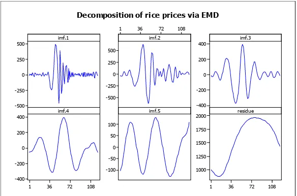
Basically, EMD-ARIMA is a combination of EMD and ARIMA to forecast a time series data set. Firstly, the original data set is decomposed into IMFs and residue. Figure 5 shows the decomposed data into six data sets via EMD. Next, each IMF and the residue applied the ARIMA before they are sum up together back to get the EMD-ARIMA forecasting. Figure 6 shows the framework view on how the EMD-ARIMA is done.
Figure 6: Framework of EMD-ARIMA forecasting
3.4 Accuracy criteria of forecasting
The root mean squared error (RMSE) and the mean absolute error (MAE) statistic can be as the accuracy criteria of the forecasting result for ARIMA and EMD-ARIMA. The RMSE statistics is defined as below
RMSE P∑SRTUQR Q0R *
+ (11)
and the MAE is given by
MAE +∑ |0+D. | (12)
Where is the actual value, 0 is the prediction value, and % is the total number of data.
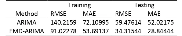
Table 1: Comparison of ARIMA and EMD-ARIMA forecasting result
Method
Training Testing
RMSE MAE RMSE MAE
ARIMA 140.2159 72.10995 59.47614 52.02175
4 Forecasting result
In this paper, all of the works were carried out by using R software which is a free software specially for statistical computing, except for some graphing figures which Minitab is used for that purpose. For the ARIMA method, after comparing several models, this paper found out that ARIMA(2,1,0) passed the diagnostic checking using the Ljung-Box statistics with all large -values, as shown in figure 4. ARIMA(2,1,0) also has the smallest value of AIC compared to other models which is 1228.23.
While the model selection for EMD-ARIMA method, each decomposed datasets are running as the same flow as the single ARIMA method was done. Later, the fitted values for every datasets are summarized to get the final fitted result. The
Table 1 shows the comparison of RMSE and MAE of both methods which are ARIMA and EMD-ARIMA. Clearly from the result, EMD-ARIMA method gives the smaller value of error for both training data set and testing data set as well. As a conclusion, this approved that the hybrid method of EMD-ARIMA is giving a strength of ARIMA and EMD in linear and nonlinear modeling. From the result, it suggests that the hybrid of EMD-ARIMA able to perform well just like the previous researchers have proved before. So far, this paper strengthen the idea that EMD-ARIMA method is suitable for crop prices forecasting. However, we believe that in the future, a new combination method will be discovered for a better idea and result.
References
[1] A. Amran, K. Assis, & Y. Remali, Forecasting cocoa bean prices using univariate time series models, Journal of Arts Science and Commerce, 1 (2010), 71-80.
[2] G.E.P. Box, & G.M. Jenkins, Time Series Analysis: Forecasting and Control, Holden-Day, San Fransisco, 1976.
[3] Hakan Adanacioglu & Murat Yercan, An analysis of tomato prices at wholesale level in Turkey: An application of SARIMA model, Custos e agronegoclo on line, 8 (2012), 52-75.
[4] M.A. Islam, M.F. Hassan, M.F. Imam, & S.M. Sayem, Forecasting coarse rice prices in Bangladesh, Progress Agriculture, 22 (2011), 193-201.
[5] N.E. Huang, S.R. Long, & Z. Shen, The empirical mode decomposition and the Hilbert spectrum for nonlinear and non-stationary time series analysis, Proceedings of the Royal Society of London A, 459 (1998), 2317-2345.
[6] C. Chen, H. Liu, H. Tian, & Y.F. Li, A hybrid model for wind speed prediction using empirical mode decomposition and artificial neural networks, Renewable Energy, 48 (2012), 545-556.
[7] G. Dinpanah, H. Alipoor, M.H. Ansari, & P.A. Pargami, Application of seasonal models in modelling and forecasting the monthly price of Privileged Sadri rice in Guilan province, ARPN Journal of Agrcultural and Biological Science, 8 (2013), 283-290.
[8] A.L. Sandika, An analysis of price behaviour of rice in Sri Lanka after liberalization of economy, Tropical Agricutural Research & Extension, 12 (2009).
[9] D.M. Tuong, Analysis marketing and forecasting rice price in the Mekong Delta of Vietnam, Omonrice, 18 (2011), 182-188.
[11] X. Xu, Y. Qi, & Z. Hua, Forecasting demand of commodities after natural disasters, Expert Systems with Applications, 37 (2010), 4313-4317.
[12] G.P. Zhang, Time series forecasting using a hybrid ARIMA and neural network model, Neurocomputing, 50 (2003), 159-175.