A New Model for Visualizing Interactions in
Analysis of Variance
Patrick J.F. Groenen
Alex J. Koning
∗February 13, 2004
Econometric Institute Report EI 2004-06
Abstract
In analysis of variance, there is usually little attention for inter-preting the terms of the effects themselves, especially for interaction effects. One of the reasons is that the number of interaction-effect terms increases rapidly with the number of predictor variables and the number of categories. In this paper, we propose a new model, called the interaction decomposition model, that allows to visualize the interactions. We argue that with the help of the visualization, the interaction-effect terms are much easier to interpret. We apply our method to predict holiday spending1 using seven categorical predictor variables.
1
Introduction
In many situations of empirical research, there is the need to predict a nu-merical variable by one or more categorical variables. In its most simple case, the question is posed whether two groups of persons or subjects have
a different mean or not, which can be answered by a simple t-test. Here, we
call the numerical variable of interest is called the dependent variable and the grouping variable a predictor variable. If the number of groups is larger than two, we would like to know whether the means between the groups are all the
∗Econometric Institute, Erasmus University Rotterdam, The Netherlands
same or not. In this situation analysis of variance can be used. As soon as there are two or more categorical predictor variables, interaction effects may turn up. If so, then different combinations of the categories of the predictor variables have different effects. The majority of the papers in the literature only report an ANOVA table showing which effect is significant, but do not present or interpret the terms belonging to the effects themselves.
Each effect is characterized by a number of terms depending on the
cat-egories involved. For example, a main effect is characterized by Kj terms,
where Kj is the number of categories of predictor variable j. In this
pa-per, we argue that it is worthwhile to consider the terms that constitute the effects directly. Doing so may be difficult if the number of categories and the number of categorical predictor variables grows, because the number of interaction-effect terms will also grow dramatically. Therefore, we describe a new interaction decomposition model that allows two-way interactions to be visualized in a reasonably simple manner. The interpretation of the in-teraction plot is similar to that of correspondence analysis. Although in principle, the method could be used to analyze higher-way interactions, we limit ourselves to two-way interactions only.
The remainder of this paper is organized as follows. First, we discuss the empirical data set on predicting holiday spending in some detail and apply a common ANOVA. Then, we explain the interaction decomposition model more formally. We continue by applying our model to the holiday spending data set. We end this paper with some concluding remarks.
2
Holiday Spending Data
In this section, we discuss the empirical data set that we use in this paper. The data concern the holiday spending of 708 respondents. The data were gathered by students of the Erasmus University Rotterdam in 2003. The purpose of this research is to predict the amount of holiday spending in eu-ros out of seven categorical predictor variables, that is, number of children, income, destination, other big expenses, accommodation, transport, and hol-iday length. Table 1 gives the frequencies of each of the categories of the predictor variables. Most categories are reasonably filled, with the exception of number of children, where almost 80% of the respondents has no children, whereas the other 20% has one to five children.
4 5 6 7 8 9 10 0
20 40 60 80 100 120 140
log(holiday spending)
Frequency
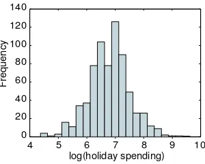
Figure 1: Histogram of the natural logarithm of the holiday spending.
The reason for this to happen is that there will always be a few people in a sample that are able to spend much more money on a holiday than the middle 50%. Such skewness is quite common in economics for variables like price, income, and spending in general. Cram´er (1946, p. 220) remarks
“Consider the distribution of incomes or property values in a certain population. The position of an individual on the property scale might be regarded as the effect of a large number of impulses, each of which causes a certain increase of his wealth. It might be argued that the effect of such an impulse would not unreasonably be expected to be proportional to the wealth already attained. If this argument is accepted, we should expect distributions of incomes or property values to be approximately log-normal.”
To make the variable less skewed and more like a normal distribution, we take the logarithm of the holiday spending. The histogram of log holiday spending is given in Figure 1. Indeed, the logarithm transformation has made the variable behave much more like a normal distribution. Thus, throughout this paper, log holiday spending will be the dependent variable.
Table 1: Frequencies and percentages of categorical predictor variables for the holiday spending data.
Number of children Freq % Income Freq %
0 children 559 79.0 <400 euro 75 10.6
1 child 49 6.9 400-800 euro 122 17.2
2 children 63 8.9 800-1600 euro 124 17.5
3 children 25 3.5 1600-3200 euro 237 33.5
4 children 11 1.6 3200-4000 euro 88 12.4
5 children 1 .1 4000- euro 62 8.8
Destination Freq % Other big expenses Freq %
Within Europe 543 76.7 No big expenses 522 73.7 Outside Europe 165 23.3 Other big expenses 186 26.3
Holiday length Freq % Accommodation Freq
<7 days 65 9.2 Camping 162 22.9
7-14 days 277 39.1 Apartment 189 26.7
14-21 days 223 31.5 Hotel 216 30.5
21-28 days 88 12.4 Other 141 19.9
>28 days 55 7.8
Transport Freq %
By car 261 36.9
conveniently as a linear sum of terms for each of the categories of the predictor variables.
However, joint effects of two predictor variables are not taken into ac-count. For our data, it may well be so that people with more children spend more and those who have longer holidays also spend more, but that the joint effect of having two or more children and have long holidays leads to less spending because a cheaper accommodation for example a camping site is
chosen. Such effects are called interaction effects. In principle, it is possible
to consider interaction effects between any number of predictor variables, but we limit ourselves to two-way interactions, that is, we only look joint effects of two predictor variables simultaneously. One important reason for doing so, is that interpreting three or higher way interactions gets increasingly more difficult.
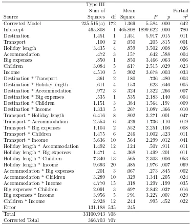
Let us look at an ANOVA on the holiday spending of the main effects and all two way interactions of the predictor variables. Almost always, the results of the ANOVA are presented in an analysis of variance table (hence the name ANalysis Of VAriance) that shows how the sum of squares of the dependent variable can be decomposed into contributions by the main and interactions effects and whether these effects are significant or not. In Table 2, these results are presented for the holiday spending data. Note that the
last column contains the partial η2, a measure for the effect size. It measures
the proportion of the variance of the dependent variable accounted for by the current factor.
From Table 2, we see that important contributors to the prediction of holiday spending are the main effects for ‘Holiday length’ and ‘Number of children’ and the interaction effects of ‘Transport’ by ‘Holiday length’, ‘Trans-port’ by ‘Income’, ‘Holiday length’ by ‘Children’, and ‘Accommodation’ by ‘Income’. A few other main and interaction effects are significant and have reasonable effect size.
However, to understand how a certain main or interaction effect affects
Table 2: ANOVA table of all main effects and all interaction effects for the holiday spending data.
Type III
Sum of Mean Partial
Source Squares df Square F p η2
Corrected Model 235.515(a) 172 1.369 5.584 .000 .642
Intercept 465.808 1 465.808 1899.622 .000 .780
Destination 1.451 1 1.451 5.917 .015 .011
Transport .100 2 .050 .205 .815 .001
Holiday length 3.435 4 .859 3.502 .008 .026
Accommodation .472 3 .157 .642 .588 .004
Big expenses .850 1 .850 3.466 .063 .006
Children 3.084 5 .617 2.515 .029 .023
Income 4.510 5 .902 3.678 .003 .033
Destination * Transport .361 2 .180 .736 .480 .003 Destination * Holiday length .611 4 .153 .623 .646 .005 Destination * Accommodation .972 3 .324 1.322 .266 .007 Destination * Big expenses .535 1 .535 2.183 .140 .004 Destination * Children 1.151 3 .384 1.564 .197 .009
Destination * Income 1.333 5 .267 1.087 .366 .010
Transport * Holiday length 6.416 8 .802 3.271 .001 .047 Transport * Accommodation 2.554 6 .426 1.736 .110 .019 Transport * Big expenses 1.104 2 .552 2.251 .106 .008
Transport * Children 1.475 6 .246 1.002 .423 .011
Transport * Income 5.636 10 .564 2.299 .012 .041
Holiday length * Accommodation 1.492 12 .124 .507 .911 .011 Holiday length * Big expenses 1.471 4 .368 1.499 .201 .011 Holiday length * Children 7.340 13 .565 2.303 .006 .053 Holiday length * Income 9.693 20 .485 1.976 .007 .069 Accommodation * Big expenses .201 3 .067 .273 .845 .002 Accommodation * Children 3.289 10 .329 1.341 .205 .024 Accommodation * Income 4.770 15 .318 1.297 .199 .035 Big expenses * Children 2.091 3 .697 2.842 .037 .016 Big expenses * Income 3.956 5 .791 3.227 .007 .029
Children * Income 2.928 12 .244 .995 .452 .022
Error 131.188 535 .245
Total 33100.943 708
effects and
6×6 + 6×2 + 6×2 + 6×5 + 6×4 + 6×3 +
+ 6×2 + 6×2 + 6×5 + 6×4 + 6×3 +
+ 2×2 + 2×5 + 2×4 + 2×3 +
+ 2×5 + 2×4 + 2×3 +
+ 5×4 + 5×3 +
+ 4×3 = 327
terms for the interaction effects summing to 28 + 327 = 355 terms to be interpreted. Clearly, this amount of terms is too much to be interpreted. Certainly, one could choose to interpret only those main effects and interac-tion effects that are significant or have a high effect size, but still the number of terms to be interpreted can be quite large, especially if the number of categories of the predictor variables or the total number number of predictor variables increases.
Another problem with interactions terms may occur if the predictor vari-ables form an unbalanced design, which generally is the case for nonexperi-mental data. Then, some of the interaction terms cannot be estimated due to the absence of relevant data.
Therefore, the reports in many studies are limited to an ANOVA table (as Table 2) only thereby ignoring the most important part of the analysis, that is, the terms of the effects themselves. The main purpose of this paper is discuss a new approach that allows to visualize the interaction effects directly. The main advantage is that the effects are easier to interpret. The next section discusses the new model more formally.
3
Decomposing Interactions
To express our interaction decomposition model more formally, we need to
introduce some notation. Let yi be the value of the dependent variable log
‘Holiday spending’ for subject i, where i = 1, . . . , n. Suppose there are m
categorical predictor variables. Each category can be presented as a dummy
variable that equals one if subject i falls in that particular category and
zero otherwise. The collection of all dummy variables for a single categorical
predictor variablej can be gathered in then×Kj indicator matrixGj, where
the categories for 6 subjects, then G is given by
Using the notation above, the main-effects model in ANOVA is given by
yi =c+
where c is the overall constant, ajk is the main-effect term for category k of
variable j, andei is the error in prediction for subject i. In matrix notation,
(1) can be simplified by denoting row i ofGj bygij′ and the main effects for
The main-effects model in ANOVA determines the main effects aj and the
constant cin such a way that the sum-of-squares of the errors ei is minimal,
that is, it minimizes the loss function
Lmain(c,a1, . . . ,am) =
where, for notational convenience, a= [a′
1, . . . ,a′m]′ contains all main-effects
terms.
To specify an interaction effect between predictor variables j and l,
con-sider the Kj ×Kl matrix Bjl that contains all the terms of the interaction
effect for all combinations of the categories of variables j and l. Suppose
that subject i falls in category k of predictor variablej and in category s of
predictor variable l. Then, the term of the interaction effect needed for this
respondent isb(jl)ks , the element in rowk and columnsofBjl. For this person
i, this element can also be picked by expression
b(jl)ks =g′
To make notation more compact, let all interaction effects be gathered in the symmetric partitioned block matrix
B=
Note that the diagonal blocks are zero because g′
ijBjjgij only selects the
diagonal and thus estimates a main effect for variablej. Because main effects
are already taken care of by aj, we choose the diagonal blocksBjj =0, since
it does not make sense to model a main effect twice.
Now, the ANOVA model with all main effects and all two-way interaction effects minimizes
The number of parameters to be estimated is 1 for the constant, Pm
j=1Kj
for the main effects in a, andPm
j=1
Pm
l=j+1Kj×Kl for the interaction effects
in Bjl. Note that some additional constraints are necessary to avoid that
interaction effects pick up main effects and the main effects pick up the constant effect. The constraints often imposed are the sum of each of the
main effects aj to be equal to zero and the interaction effects Bjl must have
row and column sums equal to zero.
We now turn to the interaction-decomposition model proposed in this
paper. The key idea of this model is that the interaction terms Bjl are
constrained such that an easy graphical representation is possible. The type of constrained used in the interaction-decomposition model is that of common rank-reduction, that is, we require that
Bjl=YjY′l, (5)
where theKj×pmatrixYj has rank not higher thanp > 0. Equivalently, we
may write that in the interaction-decomposition model an interaction term
of category k of predictor variable j and categorys of predictor variable l is
given by
b(jl)ks =y′
jkyls,
wherey′
jk denotes rowk of Yj. Using this kind of constraint, the interaction
term is graphically represented by a projection of the vector y′
Thus, high projections indicate large interaction terms, and small projections indicate small interaction terms. Such a rank restriction is also used in bi-additive models such as correspondence analysis, multiple correspondence analysis, and joint correspondence analysis. The interaction-decomposition
model has as its main advantage that there is only a single vector y′
jk to
be estimated for each category of a predictor variable. In other words, the number of interaction parameters to be estimated only grows linearly with the number of categories, and not quadratically as for the unconstrained ANOVA interaction model in (4).
Because projections do not change under rotation, the vectors in Yj are
determined up to a common rotation that is the same for all Yj. Other than
the rotation indeterminacy, the Yj’s and thus the interactions Bjl =YjYl′
can be estimated uniquely if the number of dimensions is low enough. This contrasts with standard ANOVA that cannot estimate all interaction terms, if not all combinations of predictor categories are observed.
Obviously, because the interaction-decomposition model imposes con-strains on the interactions, it will generally not fit as well as the unconstrained ANOVA interaction model in (4).
Note that we still have to require thatBjlhas zero row and column sum to
avoid confounding of the main and interaction effects. This restriction implies
that each Yj must have column sum zero so that indeed Bjl = YjYl′ will
have row and column sums equal to zero. To fit the interaction-decomposition
model, we have developed a prototype in MatLab that minimizesLint(c,a,B)
subject to the constraints (5) by alternating least-squares. The details of this algorithm are beyond the scope of this paper and will be published in subsequent papers.
For two categorical predictor variables, similar decomposition models were proposed in the literature (Eeuwijk, 1995; De Falguerolles & Francis, 1992; Gabriel, 1996; Choulakian, 1996). In psychometrics, such a models has been known under the name FANOVA (Gollob, 1968). A different way for modelling three-way interactions among three categorical predictors was pre-sented by Siciliano and Mooijaart (1997). The difference with our approach is that we limit ourselves to two-way interactions only. We believe that two way interaction convey the most important information while they are still reasonably easy to interpret. For three or higher way interactions, the inter-pretation becomes far more difficult. Another difference with previous mod-els in the literature is that our model is that the interaction-decomposition model is not limited to two or three we categorical predictor variables, but we can handle any number of predictors.
Greenacre, 1984; Gifi, 1990). Similar to joint correspondence analysis, the
diagonal effects of Bjj are simply discarded. However, the main difference
lies in the fact that the main effects in joint correspondence analysis are not
linearly modelled by separate terms g′
ijaj, but are included as weights in the
loss function. A minor difference consists in different normalization of the
Yj.
4
Interaction Decomposition of Holiday
Spend-ing
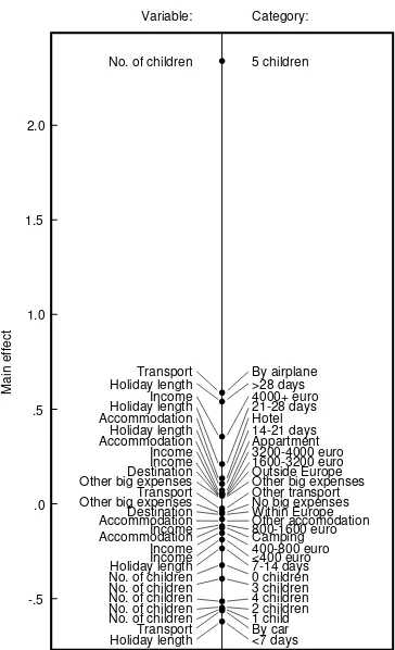
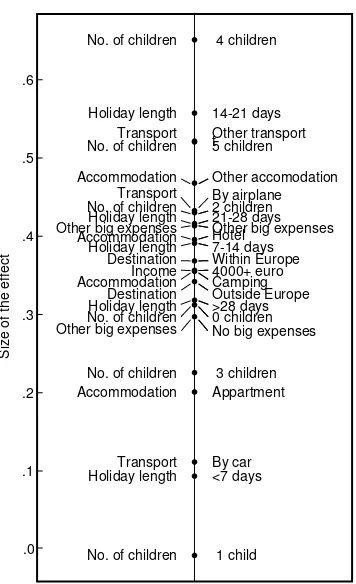
Let us apply the interaction decomposition model to the holiday spending data. First, we consider the main effects for all the categories (see Figure 2). The most striking feature is the large main effect of ‘5 children’. From Table 1 we know that there was just a single family with 5 children in this data set. Apparently, this family has spent much more money on their holiday in comparison to the rest, because it has a large positive main effect that predicts more money to be spent during the holiday. Here we choose to interpret only effects larger than plus or minus .2. Since the dependent variable is the logarithm of holiday spending, effects larger than .2 imply
that the holiday spending goes up by a factor exp(.2) = 1.22 thus increases
by 22%. Apart from the category ‘5 children’, we see that more money is spent if the travel takes place by airplane, for holidays longer than 21 days, and if the income is 4000 euros or higher. On the other hand, holiday spending reduces for holidays shorter than 7 days and –to a lesser extent– from 7 to 14 days, made by car, if there are zero to four children, and if the income is lower than 800 euros. The other main effects are reasonably small, suggesting that they are not very important.
-.5 .0 .5 1.0 1.5 2.0
Destination Outside Europe
Transport By car
Transport By airplane
Transport Other transport
Holiday length <7 days
Holiday length 7-14 days
Holiday length 14-21 days
Holiday length 21-28 days
Holiday length >28 days
Accommodation Camping
Accommodation Appartment
Accommodation Hotel
Accommodation Other accomodation
Other big expenses No big expenses
Other big expenses Other big expenses
No. of children 0 children
No. of children 1 child
No. of children 2 children
No. of children 3 children
No. of children 4 children
No. of children 5 children
Income <400 euro
Income 400-800 euro
Income 800-1600 euro
Income 1600-3200 euro
Income 3200-4000 euro
Income 4000+ euro
Category:
Main effect
Destination Within Europe
Variable:
-1.2 -.8 -.4 0 .4 .8 <400 euro 800-1600 euro
4000+ euro
Within Europe Outside Europe
Other
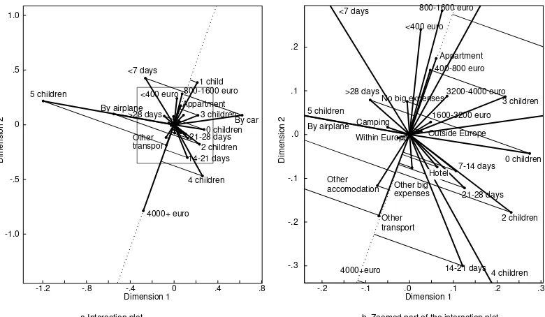
a.Interaction plot. b. Zoomed part of the interaction plot.
Dimension 2
Hotel
Figure 3: Interaction plot for the interaction decomposition model on the holiday spending data. Panel (b) zooms in on the part of the box in Panel (a) to view the labels more clearly.
are long enough. An example of this case is the interaction effect between ‘5 children’ and Income ‘4000+ euro’, which is still reasonable. Also, long vectors generally have larger interaction with all other categories.
Note that variables with only two categories will have equal length vectors that are mirrored in the origin. In Figure 3b, we see an example of this case for variable ‘Other big expenses’ (with categories ‘No big expenses’ and ‘Other big expenses’). The reason for two equal length and opposite vectors lies in the restriction that the coordinates have zero column sum per variable. For a two category variable, this restriction implies equal but mirrored vectors for the categories.
-1.2 -.8 -.4 0 .4 .8 <400 euro 800-1600 euro
4000+ euro
Within Europe Outside Europe
Other
a.Interaction plot. b. Zoomed part of the interaction plot.
Dimension 2
Hotel
Figure 4: Interaction decomposition plot with projections onto the category ‘Income 4000 or more’. Panel (b) shows the part in the box of Panel (a) to present the labels more clearly.
euro’, the holiday spending decreases if there are only one or three children, the holiday length is less than seven days, the trip is made by car, and the accommodation is an appartement. In general, a plot as in Figure 5 is very helpful in interpreting the interaction terms conditioned on a certain cate-gory.
The most important interactions can also be derived directly from Figure 3 by looking at the largest vectors. The categories that matter most in the interactions are families of 0, 1, 4, and 5 children, holidays shorter than 7 days, having one child, using the car or the airplane as means of transporta-tion. For example, for holidays shorter than 7 days, the model predicts higher spending if there is one child (because the vectors project highly) and lower spending if there are four children (because the vectors project negatively). Logically, holiday spending also increases for holidays shorter than 7 days made by air plane, but decreases if the holiday is done by car.
.0 .1 .2 .3 .4 .5 .6
Destination Within Europe
Destination Outside Europe
Transport By car By airplane Transport
Transport
Other transport t
Holiday length <7 days Holiday length 7-14 days Holiday length 14-21 days
Holiday length 21-28 days
Holiday length >28 days Accommodation Camping
Accommodation Appartment Accommodation Hotel
Accommodation Other accomodation
Other big expenses No big expenses Other big expenses Other big expenses
No. of children 0 children
No. of children 1 child No. of children 2 children
No. of children 3 children No. of children 4 children
No. of children 5 children
Income 4000+ euro
Size of the effect
5
Conclusions
To investigate interactions in the traditional ANOVA framework, most re-searchers limit themselves to an ANOVA table. We have argued in this paper that it is worthwhile to study the interaction term themselves. Because the number of interaction terms increases rapidly with the number of categorical predictor variables and the number of categories per variable, we have pro-posed a new model, called the interaction decomposition model, that allows to visualize the interactions.
In principle, the current model can be extended to Generalized Linear Models (Nelder & Wedderburn, 1972; McCullagh & Nelder, 1989). It remains to be seen if the present model needs to be adapted or not.
References
Choulakian, V. (1996). Generalized bilinear models. Psychometrika, 61,
271–283.
Cram´er, H. (1946). Mathematical methods of statistics. Princeton, N. J.:
Princeton University Press.
De Falguerolles, A., & Francis, B. (1992). Algorithmic approaches for fitting
bilinear models. In Y. Dodge & J. Whittaker (Eds.), Compstat 1992
(p. 77-82). Heidelberg: Physica-Verlag.
Eeuwijk, F. A. (1995). Multiplicative interaction in generalized linear models.
Biometrics, 85, 1017–1032.
Gabriel, K. R. (1996). Generalised bilinear regression. Biometrika,85, 689–
700.
Gifi, A. (1990). Nonlinear multivariate analysis. Chichester: Wiley.
Gollob, H. F. (1968). A statistical model which combines features of factor
analytic and analysis of variance techniques. Psychometrika, 33,
73-116.
Greenacre, M. J. (1984). Theory and applications of correspondence analysis.
New York: Academic Press.
Greenacre, M. J. (1988). Correspondence analysis of multivariate categorical
McCullagh, P., & Nelder, J. A. (1989). Generalized linear models. London: Chapman and Hall.
Nelder, J. A., & Wedderburn, R. W. M. (1972). Generalized linear models.
Journal of the Royal Statistical Society A, 135, 370–384.
Siciliano, R., & Mooijaart, A. (1997). Three-factor association models for
three-way contingency tables. Computational Statistics and Data