Integration of feedforward neural network and finite element in the draw-bend springback prediction.

(1)

Integration of feedforward neural network and finite element

in the draw-bend springback prediction

M.R. Jamli

a,b,⇑

, A.K. Ariffin

a

, D.A. Wahab

a

a_{Department of Mechanical and Materials Engineering, Faculty of Engineering and Built Environment, Universiti Kebangsaan Malaysia, 43600 UKM Bangi, Selangor, Malaysia} b_{Department of Manufacturing Process, Faculty of Manufacturing Engineering, Universiti Teknikal Malaysia Melaka, Hang Tuah Jaya, 76100 Durian Tunggal, Melaka, Malaysia}

a r t i c l e

i n f o

Keywords: Finite element Neural network Nonlinear elastic recovery Springback prediction

a b s t r a c t

To achieve accurate results, current nonlinear elastic recovery applications of finite element (FE) analysis have become more complicated for sheet metal springback prediction. In this paper, an alternative modelling method able to facilitate nonlinear recovery was developed for springback prediction. The nonlinear elastic recovery was processed using back-propagation networks in an artificial neural network (ANN). This approach is able to perform pattern recognition and create direct mapping of the elastically-driven change after plastic deformation. The FE program for the sheet metal springback experiment was carried out with the integration of ANN. The results obtained at the end of the FE analyses were found to have improved in comparison to the measured data.

1. Introduction

Sheet metal forming has been used widely in the manufacturing industry, especially in the automotive manufacturing sector. One of the main problems faced in the sheet metal forming process is the springback phenomenon. The occurrence of springback after the formation process results in inaccuracy of the final dimensions for a particular product. For decades, springback prediction tech-niques have been studied using the finite element (FE) method to replace the testing (trial and error) procedure in order to reduce the time and cost of analysis. Prediction by the FE method requires a deep knowledge of several factors that influence the final result of the analysis such as the friction coefficient, mesh density, mate-rial constitutive model, and so on. The matemate-rial constitutive model is one of the most important factors that influence the accuracy of sheet metal springback prediction by the FE method (Eggertsen & Mattiasson, 2011). Although proper utilisation of yield criteria and hardening laws is essential to accurately reproduce the mate-rial flow stress, the accuracy of the simulation of elastic unloading behaviour remains a significant factor for the end result of sheet metal springback. This is due to the nonlinearity of elastic unload-ing that occurs durunload-ing the sprunload-ingback process after the formunload-ing load is released from the metal strips.

The development of an additional surface in the yield surface (Eggertsen & Mattiasson, 2010b) and the transition of the elastic

to the plastic model (Quasi-Plastic–Elastic model) (Sun & Wagoner, 2011) have been proposed for the description on nonlinear elastic recovery in constitutive modelling. However, due to the complex-ity of developing the nonlinear recovery model, the variable elastic modulus achieves a relatively wider range of application in spring-back predictions (Chatti & Hermi, 2011; Zhu, Liu, Yang, & Li, 2012). An artificial neural network (ANN) is a mathematical model that attempts to mimic the large amount of interconnections of the bio-logical neurons in the human brain to perform a complex process-ing task. The behaviour of complex experimental data can be predicted by developing a neural network model with sufficient in-put data. In the past years, the applications of ANN in the field of sheet metal forming have been used as inverse techniques by uti-lising FE analysis to predict parameters for established constitutive models.Aguir, BelHadjSalah, and Hambli (2011)proposed a hybrid optimization strategy based on an FE method, ANN computation, and genetic algorithm (GA) to identify the Karafillis and Boyce cri-terion, and the Voce law hardening parameters.Aguir, Chamekh, BelHadjSalah, Dogui, and Hambli (2008)used ANN to identify the parameters which reduce the difference between the FE method and the experimental measurements.Veera Babu, Ganesh Naraya-nan, and Saravana Kumar (2010)developed an ANN model to pre-dict the deep drawing behaviour using a large set of data from simulation trials. Kazan, Firat, and Tiryaki (2009) investigated springback in the wipe-bending process, developing an ANN model based on data obtained from FE analysis.

Instead of utilising FE to provide training data, ANN models have also been used for mapping input and output parameters based on a large set of experimental measurements. Baseri, Bakhshi-Jooybari, and Rahmani (2011) proposed a new fuzzy

http://dx.doi.org/10.1016/j.eswa.2013.12.006

⇑Corresponding author at: Department of Manufacturing Process, Faculty of Manufacturing Engineering, Universiti Teknikal Malaysia Melaka, Hang Tuah Jaya, 76100 Durian Tunggal, Melaka, Malaysia. Tel.: +60 63316019; fax: +60 63316411.

E-mail address:ridzuanjamli@utem.edu.my(M.R. Jamli).

Contents lists available atScienceDirect

Expert Systems with Applications

(2)

learning back-propagation (FLBP) algorithm to predict the spring-back. The model was trained using the data generated based on experimental observations. Narayanasamy and Padmanabhan (2010) compared regression modelling and ANN for predicting springback in a steel sheet. In other metal-forming fields, there are several reports on the application of ANN to model complex constitutive models without any implementation of ANN-based constitutive models in FE code (Ji, Li, Li, Li, & Li, 2010; Jing, 2011; Lin, Zhang, & Zhong, 2008;Lu et al., 2011; Sun et al., 2010; Toros & Ozturk, 2011; Zhu, Zeng, Sun, Feng, & Zhou, 2011).

The disadvantages of the FE inverse technique are that the end results are limited to the FE code capability, and a large number of simulation data are required. On the other hand, ANN prediction that is based on experimental measurements cannot be used in the FE simulation. At the same time, a large number of experimen-tal data are required, resulting in a high experimenexperimen-tal cost. These problems can be solved by utilising ANN as a constitutive model or a part of it in an FE analysis. In the wide engineering spectrum, several researchers have implemented it in their works (Haj-Ali & Kim, 2007; Yun, Ghaboussi, & Elnashai, 2008a; Yun, Ghaboussi, & Elnashai, 2008b).Jung and Ghaboussi (2006)reported the formula-tion of a rate-independent ANN-based material model for concrete and its implementation in FE software through a user-defined material subroutine (Abaqus-UMAT). Kessler, El-Gizawy, and Smith (2005)developed an ANN based material model for 6061 aluminium in the FE analysis of metal forging process through a user-defined material subroutine (Abaqus-VUMAT). Despite these applications, the technique has not yet been applied in the nonlin-ear recovery of sheet metal springback.

The objective of this paper is to develop a model that can predict the nonlinear elastic recovery through a soft computing approach, and that will be practically useful as part of a material constitutive model in FE analysis. In the present work, an ANN model is devel-oped to predict the relationship of the nonlinear unloading modu-lus after a range of plastic pre-strains. The trained network model is integrated with the FE code through a user-material subroutine. The accuracy of the present work was validated with simulation re-sults of the draw-bend springback test.

2. Principle of nonlinear elastic recovery

Most of the current FE method practises still utilise classic elas-toplasticity theory, which assumes that the unloading modulus after plastic deformation is parallel to the initial Young’s modulus (E0). However, several investigations have shown that the unload-ing modulus is influenced by accumulated plastic strain (Andar, Kuwabara, Yonemura, & Uenishi, 2010; Cleveland & Ghosh, 2002; Eggertsen & Mattiasson, 2009a, 2009b; Li, Yang, Wang, Bao, & Li, 2002; Yang, Akiyama, & Sasaki, 2004; Yoshida, Uemori, & Fujiwara, 2002). A decreasing unloading modulus with increasing pre-strain can be observed with a given saturated value after a large

pre-strain is applied. The degradation of the unloading modulus with respect to the plastic pre-strain is represented by an exponen-tial formula which is known as the chord modulus (Eav). This for-mula was further used by several studies to produce more accurate springback prediction results (Chatti, 2010; Eggertsen & Mattiasson, 2009a, 2009b, 2010a, 2010b, 2010c; Yoshida & Uemori, 2003; Yu, 2009)

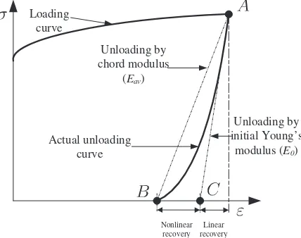
AlthoughEavhas been widely used by many researchers, several investigations have found that the unloading stress–strain curve actually shows nonlinear elastic recovery (Andar et al., 2010; Cleveland & Ghosh, 2002; Cáceres, Sumitomo, & Veidt, 2003). Fig. 1shows the nonlinear unloading stress–strain curve with re-spect toErandEav. After plastic deformation to pointA, the

unload-ing process begins at pointAand ends at pointCaccording toE0, which describes the linear elastic recovery. On the other hand, the application ofEavresults in pointBas the end of the unloading process. However, the nonlinear curveABis the actual unloading path that describes nonlinear recovery. To obtain an accurate springback prediction, the simplification of the nonlinear recovery is adequate if the springback phase achieves a relaxation in the to-tal stresses. Nevertheless, generally at the end of the springback phase, the stresses produced in the forming phase decrease but remain as residual stresses, which confirms the requirement for nonlinear recovery modelling in springback predictions (Eggertsen & Mattiasson, 2010b).

3. Methodology

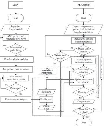
To generate the link between FE code and ANN, the application of ANN was split into the curve regeneration and interpolation coefficient parts, as shown in Fig. 2. A new curve was generated Nomenclature

FE finite element

ANN artificial neural network GA genetic algorithm E0 initial Young’s modulus

Eav chord modulus/variation of unloading modulus Ec current elastic modulus

r

1/r0 stress normalisation point

r

1 current stress

r

0 current yield stress Ce interpolation coefficient

r

true stress

s

shear stress e true strain

c

shear strain

k Lamé’s first parameter

l

shear modulus

E elastic modulus

m

Poisson’s ratio Fb back force

Loading curve

Actual unloading curve

Unloading by chord modulus

(Eav)

Unloading by initial Young’s

modulus (E0)

Nonlinear recovery

Linear recovery

(3)

from the raw experimental data, and the output was used as an in-put to the interpolation coefficient part. In both parts, the ANN was trained to learn the relationship between the input and output of nonlinear recovery. To predict the output within a desired range of errors, the number of neurons in the hidden layer was adjusted according to a number of trials. This procedure is discussed further in the next subsection.

3.1. The database and its regeneration

This study utilised the experimental data that have been pub-lished bySun and Wagoner (2011). The published data were cho-sen based on their comprehensiveness in providing information from the identification of material parameters until the measure-ments of springback. Fig. 3 shows the tensile test result for a DP980 steel sheet with intermediate unloading cycles. Due to the nonlinear unloading and reloading behaviour, hysteresis loops were formed. These loops are noticeable significantly as the flow stresses increase prior to unloading.Fig. 4(a) shows a magnified view of the fourth cycle fromFig. 3. AnEavof 145 GPa and anE0 of 208 GPa are shown for comparison. It is shown that the current

elastic modulus (Ec) varied at different stress normalisation points (r1/r0), where

r

1and

r

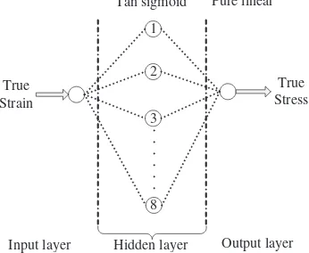
0are given by the current stress and cur-rent yield stress.Fig. 4(b) shows the regeneration of the unloading curve by the first ANN, whose architecture is shown inFig. 5. The true strain and true stress are the input and output of the network

ANN FE Analysis

Start Start

Input data (experimental)

ANN predicts and regenerate new curve

Over fitting/ under fitting

Calculate elastic modulus

Interpolate elastic modulus

ANN predicts interpolation results

Converged?

Extract neuron weights Yes

No

Yes No

Input data (geometry, applied load, initial and

boundary condition)

Increase the applied load incrementally

Calculate plastic hardening modulus Whole load

applied?

Unloading/ reloading

Update new elastic modulus, Ec

Converged?

Whole load applied?

Stop Input data

Feedforward

Output result

Exceed yield stress?

Iteration loop

Load increment loop

Output result

Yes Yes Yes Yes

No

No No

No

Yes User-defined

subroutine

Fig. 2.The establishment of the ANN model to constitutive model link in finite element software.

0 200 400 600 800 1000 1200

0 0.02 0.04 0.06 0.08 0.1

True Strain

See fig. 4(a)

(4)

with eight neurons in the single hidden layer. In both networks, the hyperbolic tangent sigmoid transfer function (tan sigmoid) was chosen as the activation function in the hidden layer due to its abil-ity to learn faster (Haykin, 1999).

3.2. Determination of interpolation coefficient

In the second ANN, the input and output data of the network were formed based on the regenerated curve inFig. 4(b). An inter-polation model was applied to interpolate the range betweenEav andE0at every

r

1/r0, as shown in Eq.(1).

Ce¼

EcEav

E0Eav

ð1Þ

where

r

1/r0andCeare the input and output of the network train-ing.Fig. 6shows the second ANN architecture with 16 neurons in the single hidden layer. At the end of the second ANN prediction, the weights of the neurons in the network were extracted as matri-ces. These matrices were then used to establish the ANN link in the FE procedure.

3.3. Establishment of ANN to FE analysis link

The second ANN was completely trained, and the neuron’s weights and biases were extracted in the form of matrices. A feed-forward network from the matrices was implemented into the user-defined material subroutine, as a portion of the material con-stitutive model used by the FE code in the structural analysis. The feedforward network takes place when the unloading/reloading process occurs after loading in the plastic region. In the FE model, the whole steel sheet was assumed to be a three-dimensional

isotropic linearly elastic body (Sun & Wagoner, 2011), and the stress–strain relations are given as:

r

x

r

y

r

z

s

x

s

y

s

z 8 > > > > > > > > < > > > > > > > > : 9 > > > > > > > > = > > > > > > > > ; ¼

kþ2

l

k k 0 0 0

k kþ2

l

k 0 0 0

k k kþ2

l

0 0 0

l

0 0

0 0 0 0

l

0

0 0 0 0 0

l

2 6 6 6 6 6 6 6 6 4 3 7 7 7 7 7 7 7 7 5

e

x

e

y

e

z

c

x

c

y

c

z 8 > > > > > > > > < > > > > > > > > : 9 > > > > > > > > = > > > > > > > > ;

ð2Þ

where the Lamé’s constantskand

l, are related to the modulus of

elasticityEand the Poisson’s ratio

m

by:

k¼ E

v

ð1þ

v

Þð12

v

Þ ð3Þ

and

l

¼ E

2ð1þ

v

_Þ ð4Þ

In the elastic region, both the unloading and the reloading processes only utiliseE0to determine the stress of the tensor, whereas varia-tion occurs in those processes in the plastic region. As shown in Fig. 4(a), Ec produces a hysteresis loop that lies between E0 and Eav. Therefore, in FE analysis,Ecneed to be updated at every incre-ment of the unloading/reloading process. The function of the feed-forward-network-based constitutive model in an FE model at every increment is as follows:

(i) For the (i+ 1)th strain increment, the input of the network is the value of

r

1/r0. To distinguish the input between unload-ing and reloadunload-ing processes, the input is expressed as (1

r

1/r0) and (r1/r0).

(ii) Ecis then calculated by reversing Eq.(1)as:

Ec¼Ce ðE0EavÞ þEav ð5Þ

3.4. Draw-bend springback test and simulation

The developed model was then utilised in the simulations of the draw-bend springback test based on the experimental works (Sun & Wagoner, 2011). The published experimental work was chosen based on its capability to represent a wide range of sheet metal forming operations while also having the advantage of simplicity and a controllable sheet tension force.Fig. 7shows a schematic of the draw-bend test that was utilised to mimic the mechanics in sheet metal forming, which consist of drawing, tensioning, bending, and straightening when passing over the die radius. The strip was cut to a width of 25 mm along the rolling direction, and lubricated with stamping lubricant. There are two hydraulic 0 200 400 600 800 1000 1200

0.069 0.074 0.079

T

rue Stress (MPa)

True Strain 208GPa 145GPa 0 200 400 600 800 1000 1200

0.069 0.074 0.079

T

rue Stress (MPa)

True Strain Source

Regenerated curve

(a)

(b)

Fig. 4.(a) Magnified view of the fourth unloading–reloading withE0andEav(Sun and Wagoner, 2011), and (b) new unloading curve regenerated by the first ANN.

True Strain

True Stress

Input layer Hidden layer Output layer

Pure linear Tan sigmoid 1 2 3 8

Fig. 5.Neural network architecture for curve regeneration.

(5)

actuators (upper & lower) oriented at 90°to each other and a rotat-ing cylinder with a radius of 6.4 mm was located at the action line intersection. The purpose of the rotating cylinder was to simulate the radius of the die where the strip will go through the drawing process. The upper actuator was used to generate a constant con-trolled force or back force (Fb), whereas the lower actuator was dis-placed at a constant velocity to draw the strip through the rotating cylinder. The drawing process was started when the lower actuator was displaced to 127 mm at a velocity of 25.4 mm/s. At the same time, the upper actuator was applied withFbwhich was set to be 30 to 80% from the 0.2% offset of the yield strength. At the end of the drawing process, the strip was released from the grippers and fixtures to allow springback of the drawn strip.

The draw-bend springback test simulation used a three-dimensional FE model with an implicit solver for the bending, drawing, and springback steps as shown inFig. 8(a)–(c). In the sim-ulation,E0and

m

were 208 GPa and 0.291, respectively. The plastic deformation process (hardening) was assumed to be isotropic and the plastic modulus was generated based on a monotonic curve as shown inFig. 3. The coefficient of friction between the strip surface and the rotating cylinder was set to be 0.04 in the simulation. Fig. 8(a) represents the position of the strip after a simple bending step to obtain the initial L-shape.Fbwas applied at the left end of the strip to create controlled pre-tension in every element of the strip model.Fig. 8(b) shows the simulation of the fully drawn strip after the total displacement boundary was applied to the right

end of the strip. To simulate the final shape of the strip, all con-straints on the strip were released to allow it to springback, as shown inFig. 8(c).

4. Results and discussion

The purpose of regenerating the unloading curve was to gener-alise the determination of the elastic modulus at every

r

1/r0, as shown inFig. 9(a). This determination was used as the training data set for the prediction ofCe. If the number of neurons is exces-sive, the network may generate near perfect matching (over-fitted) of the output to the target, as shown inFig. 9(a), while the insuffi-cient number of neurons may generate an imprecise unloading curve that affects the accuracy of FE simulation.Fig. 9(b) shows the performance of the network training according to the number of neurons in the hidden layer. Although the mean squared error (MSE) value keep on decreasing with the increasing number of neurons, the suitable network was found to have eight neurons only. This is due to the consideration of the network architecture of the second ANN that was influenced by the first ANN perfor-mance. Fig. 10 shows a comparison of the training data set for the second ANN with respect to the first ANN architecture. A single neuron results in a near straight line, and the increasing number of neurons produce curved data sets. With eight neurons, the net-work results in quite a smooth curve. However, as the number of neurons increased, the network generates higher fluctuations, which affect the prediction difficulty in the second ANN.

In the interpolation coefficient part, the second ANN architec-ture was similar to the curve fitting part except for the number of neurons in the hidden layer. In this part, high accuracy is essen-tial as the result was utilised directly in the FE analysis. Therefore, the number of neurons in the hidden layer was chosen according to the network performance.Fig. 11(a) shows the performance of the trained network at a various number of neurons. It can be observed that the MSE decreased with the increasing number of neurons and reached a value of 1.75e5_{with 16 neurons. This performance is} adequate since the training regression reached a value of 0.99998, as shown inFig. 11(b).

As shown inFig. 3, the hysteresis loops are noticeable signifi-cantly as the flow stresses increase prior to unloading. This was due to the variation ofEavat each unloading path. Since the network training set was taken from a single hysteresis loop, the interpola-tion model as shown in Eq.(1)represents its behaviour according to the particularEav andE0. Therefore, once the model has been trained by the second ANN, its prediction could be used in modelling the unloading process at different initial unloading points.

The establishment of an ANN to FE analysis link utilised the for-mation of matrix multiplication in the user-material subroutine, where the matrices were the neuron’s weights and biases that were extracted from network training. Therefore, the sizes of the matri-ces depend on the number of neurons used for the prediction. This consideration was significant as the matrix multiplications were in-cluded into the user material subroutine manually. The neurons in the hidden layer calculate the weighted sum of inputs and bias as shown in Eq.(6), and its outputs were passed through the transfer function in Eq.(7)as an input (U1,U2,. . .,U16) to the output layer.

U1 U2 . . . U16 2 6 6 6 6 4 3 7 7 7 7 5 ¼tanh

w11

w12

. . .

w116 2 6 6 6 6 4 3 7 7 7 7 5

½Input þ

b11

b12

. . .

b116 2 6 6 6 6 4 3 7 7 7 7 5 0 B B B B @ 1 C C C C A

ð6Þ

tanhðxÞ ¼ 2

1þe2x1 ð7Þ

Stress Normalisation

point

Interpolation coefficient

Input layer Hidden layer Output layer Pure linear Tan sigmoid 1 2 3 16

Fig. 6.Neural network architecture for the interpolation coefficient prediction.

grip gr ip Bending, unbending and friction Finish Start Start Finish V=25.4 mm/s Stroke=127 mm Final shape

(6)

At the end of the network, the output neuron receives input signals from the hidden layer and computes the weighted sum as shown in Eq.(8), thus producing the final outputCe.

Ce¼½w21;1 w21;2 . . . w21;16 U1

U2

. . .

U16 2

6 6 6 6 4

3

7 7 7 7 5

þ ½b21 ð8Þ

Fig. 12 shows the progression of Ec according to the plastic pre-strain and

r

1/r0, and a single Eav curve. It can be seen that the degradation of the elastic modulus due to the plastic pre-strain varied based on the normalised stress point. This variation is the major contribution to the formed hysteresis loop, as shown in Fig. 4(a), whereasEavcurve only results in a single exponential deg-radation.Fig. 13shows a comparison of the overall fit obtained by the FE analysis using the current model with the experimental data. Although the network training was based on the fourth cycle, the Fig. 8.Draw-bend simulation (a) obtaining the initial L-shape by simple bending, and (b) end position of the sheet drawn over the tool, (c) constraints released and springback.

0 200 400 600 800 1000 1200

0.069 0.074 0.079

T

rue Stress (MPa)

True Strain Experimental curve

Regenerated curve

0 10 20 30 40 50 60 70

0 2 4 6 8 10 12 14

Mean squared error(MSE)

Number of neurons Over-fitted

(a)

(b)

(7)

overall prediction fit obtained was adequate. It is shown that the unloading elastic modulus varied with respect to the plastic pre-strain and the stress normalisation point.

Fig. 14(a)–(c) shows the distribution of the elastic modulus after the springback step. At the end of the springback step, the elastic modulus at the plastically deformed zone experiences significant drop in the elastic modulus, whereas the elastic modulus at both ends of the strip indicates that those regions may be considered as the elastically deformed zone. Furthermore, the elastic modulus varied at different area in the plastically deformed zone. This var-iation is due to the anticlastic behaviour which contributes to a dif-ferent normalised stress point for each element after the springback step, which remains as residual stresses. For compari-son, Fig. 14(d) shows the distribution of Eav for the plastically

deformed zone. The uniform distribution of the elastic modulus is the major error contribution to the draw-bend springback test simulation.

Table 1andFig. 15show the results of springback prediction with respect to different types of unloading moduli. All prediction results were compared with the experimental results (Sun & Wag-oner, 2011), which show that the springback angle of the strip de-creases with increasing back force. The standard deviations were calculated as follows:

h

r

i ¼

ffiffiffiffiffiffiffiffiffiffiffiffiffiffiffiffiffiffiffiffiffiffiffiffiffiffiffiffiffiffiffiffiffiffiffiffiffiffiffiffiffiffiffiffiffiffiffiffiffiffiffiffi PN

i¼1ðhmodelhexperimentÞ2

N

s

ð9Þ

wherehmodelis the simulated springback angle andhexperimentis the angle calculated from the experiment.N is the number of results -4

-3 -2 -1 0 1 2 3 4

0 0.2 0.4 0.6 0.8 1

Interpolation coef

ficent (%)

Normalisation point 1 neuron

8 neurons

9 neurons

Fig. 10.Training data set for the second ANN according to the first ANN architecture.

0 0.005 0.01 0.015 0.02 0.025 0.03 0.035 0.04 0.045 0.05

0 2 4 6 8 10 12 14 16 18

Mean squared error (MSE)

Number of neurons 1.75e-5

0.95 0.955 0.96 0.965 0.97 0.975 0.98 0.985 0.99 0.995 1

0 2 4 6 8 10 12 14 16 18

Correlation coefficient (R)

Number of neurons 0.99998

(a)

(b)

Fig. 11.Influence of hidden-layer neurons on the second ANN (a) performance, and (b) training regression.

30 50 70 90 110 130 150 170 190 210

0 0.02 0.04 0.06 0.08 0.1 0.12

Unloading elastic modulus(GPa)

Plastic strain Chord modulus

Fig. 12.Unloading elastic modulus evolution according to plastic prestrain.

0 200 400 600 800 1000 1200

0 0.02 0.04 0.06 0.08 0.1

True Stress (MPa)

True Strain Current work

Experimental

(8)

compared and is equal to three. The utilisation ofE0in the unload-ing process produces under estimation of the sprunload-ingback angle with a standard deviation of 4.68. The springback angles that resulted from the utilisation ofEav show a high standard deviation, three

times higher than those resulting fromE0. On the other hand, the unloading modulus determined by the current model improves the springback prediction as compared to the experimental data.

5. Conclusions

The capability of the developed model to predict the nonlinear unloading for pre-strained steel sheet and the springback of the draw-bend test has been investigated. The applicability of ANN as a part of a constitutive model in FE code has been successfully demonstrated. The application also shows the significance of emphasising the nonlinearity of the unloading modulus instead of the chord modulus, as the final product of springback will result with residual stresses. With an appropriate network architecture, the application has the capability to achieve equivalence to the available experimental data. Therefore, the current work has a high potential to be integrated with the FE software to simulate sheet metal springback phenomenon accurately.

References

Aguir, H., BelHadjSalah, H., & Hambli, R. (2011). Parameter identification of an elasto-plastic behaviour using artificial neural networks-genetic algorithm method.Materials & Design, 32, 48–53.

Aguir, H., Chamekh, A., BelHadjSalah, H., Dogui, A., & Hambli, R. (2008). Identification of constitutive parameters using hybrid ANN multi-objective optimization procedure.International Journal of Material Forming, 1, 1–4.

Andar, M. O., Kuwabara, T., Yonemura, S., & Uenishi, A. (2010). Elastic–plastic and inelastic characteristics of high strength steel sheets under biaxial loading and unloading.ISIJ International, 50, 613–619.

Baseri, H., Bakhshi-Jooybari, M., & Rahmani, B. (2011). Modeling of spring-back in V-die bending process by using fuzzy learning back-propagation algorithm.Expert Systems with Applications, 38, 8894–8900.

Cáceres, C. H., Sumitomo, T., & Veidt, M. (2003). Pseudoelastic behaviour of cast magnesium AZ91 alloy under cyclic loading–unloading.Acta Materialia, 51, 6211–6218.

Fig. 14.Elastic modulus distribution after springback; for current work (a) left end of the strip, (b) plastically deformed zone, (c) right end of the strip; for chord modulus model, and (d) plastically deformed zone.

Table 1

Springback prediction with different unloading modulus.

Fb 0.3 0.6 0.8 hh0i

Experiment (Sun and Wagoner, 2011) 63.5° 53.9° 45.9° 0

Current work 66.37° 54.55 45.94° 1.699

Initial Young’s modulus 57.7° 49.35° 42.52° 4.6821 Chord modulus 82.06° 67.66° 58.31° 15.142

40 50 60 70 80 90 100 110 120

20 40 60 80

Springback angle ( º)

Fb (%) Chord modulus

Current work

Experiment (L. Sun & Wagoner, 2011)

Initial modulus

Fig. 15.Springback prediction with different types of unloading moduli.

(9)

Chatti, S. (2010). Effect of the elasticity formulation in finite strain on springback prediction.Computers & Structures, 88, 796–805.

Chatti, S., & Hermi, N. (2011). The effect of non-linear recovery on springback prediction.Computers & Structures, 89, 1367–1377.

Cleveland, R. M., & Ghosh, A. K. (2002). Inelastic effects on springback in metals.

International Journal of Plasticity, 18, 769–785.

Eggertsen, P.-A., & Mattiasson, K. (2009a). Material modelling for accurate springback prediction.International Journal of Material Forming, 2, 793–796.

Eggertsen, P. A., & Mattiasson, K. (2009b). On the modelling of the bending– unbending behaviour for accurate springback predictions.International Journal of Mechanical Sciences, 51, 547–563.

Eggertsen, P.-A., & Mattiasson, K. (2010a). On the identification of kinematic hardening material parameters for accurate springback predictions.

International Journal of Material Forming, 1–18.

Eggertsen, P.-A., & Mattiasson, K. (2010b). On the modeling of the unloading modulus for metal sheets.International Journal of Material Forming, 3, 127–130.

Eggertsen, P.-A., & Mattiasson, K. (2010c). On constitutive modeling for springback analysis.International Journal of Mechanical Sciences, 52, 804–818.

Eggertsen, P.-A., & Mattiasson, K. (2011). Experiences from experimental and numerical springback studies of a semi-industrial forming tool.International Journal of Material Forming, 1–19.

Haj-Ali, R., & Kim, H.-K. (2007). Nonlinear constitutive models for FRP composites using artificial neural networks.Mechanics of Materials, 39, 1035–1042.

Haykin, S. S. (1999).Neural Networks: A Comprehensive Foundation. Prentice Hall International.

Ji, G., Li, F., Li, Q., Li, H., & Li, Z. (2010). Prediction of the hot deformation behavior for Aermet100 steel using an artificial neural network.Computational Materials Science, 48, 626–632.

Jing, W. (2011). Study on a Zerilli–Armstrong and an artificial neural network model for 4Cr5MoSiV1 Quenched Steel at high strain rate. In: 2011 Seventh International Conference on Natural Computation (ICNC), Vol. 1, (pp. 247–250).

Jung, S., & Ghaboussi, J. (2006). Neural network constitutive model for rate-dependent materials.Computers & Structures, 84, 955–963.

Kazan, R., Firat, M., & Tiryaki, A. E. (2009). Prediction of springback in wipe-bending process of sheet metal using neural network.Materials & Design, 30, 418–423. Kessler, B. S., El-Gizawy, A. S., & Smith, D. E. (2005). Incorporating neural network material models within finite element analysis for rheological behavior prediction. Vol. 2, (pp. 325–334).

Li, X., Yang, Y., Wang, Y., Bao, J., & Li, S. (2002). Effect of the material-hardening mode on the springback simulation accuracy of V-free bending. Journal of Materials Processing Technology, 123, 209–211.

Lin, Y. C., Zhang, J., & Zhong, J. (2008). Application of neural networks to predict the elevated temperature flow behavior of a low alloy steel.Computational Materials Science, 43, 752–758.

Lu, Z., Pan, Q., Liu, X., Qin, Y., He, Y., & Cao, S. (2011). Artificial neural network prediction to the hot compressive deformation behavior of Al–Cu–Mg–Ag heat-resistant aluminum alloy.Mechanics Research Communications, 38, 192–197.

Narayanasamy, R., & Padmanabhan, P. (2010). Comparison of regression and artificial neural network model for the prediction of springback during air bending process of interstitial free steel sheet. In Journal of Intelligent Manufacturing(pp. 1–8). Netherlands: Springer.

Sun, L., & Wagoner, R. H. (2011). Complex unloading behavior: Nature of the deformation and its consistent constitutive representation.International Journal of Plasticity, 27, 1126–1144.

Sun, Y., Zeng, W. D., Zhao, Y. Q., Qi, Y. L., Ma, X., & Han, Y. F. (2010). Development of constitutive relationship model of Ti600 alloy using artificial neural network.

Computational Materials Science, 48, 686–691.

Toros, S., & Ozturk, F. (2011). Flow curve prediction of Al–Mg alloys under warm forming conditions at various strain rates by ANN.Applied Soft Computing, 11, 1891–1898.

Veera Babu, K., Ganesh Narayanan, R., & Saravana Kumar, G. (2010). An expert system for predicting the deep drawing behavior of tailor welded blanks.Expert Systems with Applications, 37, 7802–7812.

Yang, M., Akiyama, Y., & Sasaki, T. (2004). Evaluation of change in material properties due to plastic deformation.Journal of Materials Processing Technology, 151, 232–236.

Yoshida, F., & Uemori, T. (2003). A model of large-strain cyclic plasticity and its application to springback simulation. International Journal of Mechanical Sciences, 45, 1687–1702.

Yoshida, F., Uemori, T., & Fujiwara, K. (2002). Elastic–plastic behavior of steel sheets under in-plane cyclic tension–compression at large strain.International Journal of Plasticity, 18, 633–659.

Yu, HY. (2009). Variation of elastic modulus during plastic deformation and its influence on springback.Materials & Design, 30, 846–850.

Yun, G. J., Ghaboussi, J., & Elnashai, A. S. (2008a). A design-variable-based inelastic hysteretic model for beam–column connections. Earthquake Engineering & Structural Dynamics, 37, 535–555.

Yun, G. J., Ghaboussi, J., & Elnashai, A. S. (2008b). A new neural network-based model for hysteretic behavior of materials.International Journal for Numerical Methods in Engineering, 73, 447–469.

Zhu, YX., Liu, YL., Yang, H., & Li, HP. (2012). Development and application of the material constitutive model in springback prediction of cold-bending.Materials & Design, 42, 245–258.