arXiv:0811.3832v1 [math.CO] 24 Nov 2008
Two-Dimensional Patterns with Distinct Differences
– Constructions, Bounds, and Maximal Anticodes
Simon R. Blackburn, Tuvi Etzion, Keith M. Martin and Maura B. Paterson
Abstract— A two-dimensional grid with dots is called a con-figuration with distinct differencesif any two lines which connect two dots are distinct either in their length or in their slope. These configurations are known to have many applications such as radar, sonar, physical alignment, and time-position synchronization. Rather than restricting dots to lie in a square or rectangle, as previously studied, we restrict the maximum distance between dots of the configuration; the motivation for this is a new application of such configurations to key distribution in wireless sensor networks. We consider configurations in the hexagonal grid as well as in the traditional square grid, with distances measured both in the Euclidean metric, and in the Manhattan or hexagonal metrics.
We note that these configurations are confined inside maximal anticodes in the corresponding grid. We classify maximal anti-codes for each diameter in each grid. We present upper bounds on the number of dots in a pattern with distinct differences contained in these maximal anticodes. Our bounds settle (in the negative) a question of Golomb and Taylor on the existence of honeycomb arrays of arbitrarily large size. We present constructions and lower bounds on the number of dots in configurations with distinct differences contained in various two-dimensional shapes (such as anticodes) by considering periodic configurations with distinct differences in the square grid.
I. INTRODUCTION
A
Golomb ruler(orrulerfor short) of orderm(also known as aSidon set) is a setSof integers with|S|=mhaving the property that all differencesa−b(fora, b∈S, witha6=b) are distinct. They were first used by Babcock, in connection with radio interference [5]. The length of a Golomb ruler S is the largest difference between any two elements of S. It is easy to show that a ruler of order m has length at leastm
2
; a ruler meeting this bound is called perfect. Golomb has shown that no perfect ruler exists with order greater than four [22]. The problem of finding the shortest possible length of a Golomb ruler of a given order has been widely studied; no general solution is known, but optimal rulers have been determined for orders less than 24 (see [42] for details). The elements of a Golomb ruler can be taken to represent marks (‘dots’) on a physical ruler occurring at integer differences from each other. The fact that the differences are all distinct implies that if a Golomb ruler is placed on top of a second, identical, ruler then at most one mark from the upper ruler will coincide with a mark from the lower ruler, unless they are exactly superimposed. Golomb rulers arise in the literature
This work was supported by the United States — Israel Binational Science Foundation (BSF), Jerusalem, Israel, under Grant 2006097, as well as by EPSRC grants EP/D053285/1 and EP/F056486/1.
S.R. Blackburn, K.M. Martin and M.B. Paterson are with the Department of Mathematics, Royal Holloway, University of London, Egham, Surrey TW20 0EX. T. Etzion is with the Computer Science Department, Technion–Israel Institute of Technology, Haifa 32000, Israel.
from both theoretical and practical aspects (see [4], [5], [25], [30]). It is well known that the largest order of a ruler of length nis√n+o(√n), see [4], [30], [40].
There are various generalizations of one-dimensional rulers into two-dimensional arrays. One of the most general was given by Robinson [37]. A two-dimensional ruler is ann×k array withmdots such that all m2lines connecting two dots in the array are distinct as vectors, i.e., any two have either different length or slope. These arrays were also considered in [38], [39]. The case where n = k was first considered suggested by Costas and investigated by Golomb and Tay-lor [25]. Costas considered the case when n = k and each row and each column in the array has exactly one dot [25]. These arrays have application to a sonar problem [12], [25] and also to radar, synchronization, and alignment; they are known as Costas arrays. Sonar sequences are another class of arrays mentioned in [25], wherem=kand each column has exactly one dot; see [20], [21], [34].
Other two-dimensional generalizations of a Golomb ruler have been considered in the literature, but do not have direct connection to our current work. For the sake of completeness we will mention them. A radar arrayis an n×k array with exactly one dot per column such that there are no two lines connecting two disjoint pairs of dots, occupying the same rows, which have the same length and slope. Radar arrays were defined in [25] and considered in [9], [28], [37], [45]. Arrays in which all lines have distinct slopes were considered in [14], [36], [44]. Arrays in which the Euclidean distances of any pair of lines are distinct were considered in [31].
The examples above are concerned with dots in an (infinite) square grid that are restricted to lie in a given line segment, square or rectangle. More generally, we say that a set of dots in a grid is a distinct difference configuration(DDC) if the lines connecting pairs of dots are different either in length or in slope. Having surveyed the known structures of two-dimensional patterns with distinct differences, it seems that the following natural question has not been investigated: what is the maximum number of dots that can be placed on a two-dimensional grid such that all lines connecting two dots are different either in their length or their slope and the distance between any two dots is at mostr? In other words, rather than considering the traditional rectangular regions of the square grid, we consider dots which lie in maximal anticodes of diameter r. (An anticode of diameterr is a set of positions in the grid such that any pair of positions are at distance at most r. See Section III for details.) We will consider several notions of distance: Manhattan, hexagonal and Euclidean.
sensor networks. We considered in [6] a key predistribution scheme based on DDCs in general, and Costas arrays in particular. A DDC A with m dots was shifted over the two-dimensional square grid. For each shift we assigned the same key to them entries of the two-dimensional grid which coincide with themdots ofA. In [6] we noted that a Costas array is a DDC, and gave examples of DDCs with small numbers of dots. However, the questions of finding more general constructions, and providing bounds on the number of dots in such configurations, were left open; it is these issues that are addressed by the results of this paper. Other properties of DDCs motivated by this application are considered in [7]. The rest of this paper is organized as follows. In Section II we describe the models on which we will consider our two-dimensional patterns with distinct differences. We consider two two-dimensional grids: the square grid and the hexagonal grid. In the square grid we consider the Manhattan distance and the Euclidean distance, while in the hexagonal grid we consider the hexagonal distance and the Euclidean distance. We define the classes of DDCs we will study, and list optimal examples for small parameter sizes. In Section III we explain the relation between DDCs and maximal anticodes. We classify the maximal anticodes when we use Manhattan distance and hexagonal distance. We also briefly review some properties of anticodes in R2 using Euclidean distance: these properties will allow us to bound the size of an anticode in either grid when we use Euclidean distance. In Section IV we present upper bounds on the number of dots in a DDC when we restrict the dots to lie in some simple regions (‘shapes’) in the grid. The most important shapes we consider are the anticodes, in particular the Lee sphere and the hexagonal sphere. As a consequence of our upper bound, we settle an old question of Golomb and Taylor [26] (on the existence of honeycomb arrays of arbitrarily large size) in the negative. In Sections V and VI we turn our attention to constructions and lower bounds for the number of dots in the classes of DDC defined in Section II. We generalize a folding technique that was used by Robinson [38] to construct Golomb rectangles, and provide more good examples by constructing periodic infinite arrays that are locally DDCs. Our constructions are asymptotically optimal in the case of the square grid and Manhattan distance.
II. GRIDS, DISTANCES,ANDDDCS
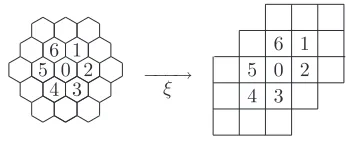
We first define some new classes of two-dimensional distinct difference configurations. We believe that the definitions are very natural and are of theoretical interest, independently of the application we have in mind. We will consider the square grid and the hexagonal grid as our surface. We start with a short definition of the two models. Before the formal definition we emphasize that we define a point (i, j)to be the point in columni and rowj of either a coordinate system or a DDC. Hence, rows are indexed from bottom to top in increasing order; columns are indexed from left to right in increasing order. (So this is the usual convention for a Cartesian co-ordinate system, but is not the standard way of indexing the entries of a finite array.)
0 56 12
4 3 −−−→ξ 5 0 2
6
4 1
3
Fig. 1. The hexagonal model translation
A. The two models
The first model is called the square model. In this model, a point(i, j)∈Z2has the following four neighbors when we consider the model as a connected graph:
{(i−1, j),(i, j−1),(i, j+ 1),(i+ 1, j)}.
We can think of the points in Z2 as being the centres of a tiling of the plane by unit squares, with two centres being adjacent exactly when their squares share an edge. The distance d((i1, j1),(i2, j2)) between two points (i1, j1) and
(i2, j2)in this model is the Manhattan distance defined by
d((i1, j1),(i2, j2)) =|i2−i1|+|j2−j1|.
The second model is called the hexagonal model. Instead of the square grid, we define the following graph. We start by tiling the plane R2 with regular hexagons whose sides have length 1/√3 (so that the centres of hexagons that share an edge are at distance1). The vertices of the graph are the centre points of the hexagons. We connect two vertices if and only if their respective hexagons share an edge. This way, each vertex has exactly six neighbouring vertices.
We will often use an isomorphic representation of the hexagonal model which will be of importance in the sequel. This representation has Z2 as the set of vertices. Each point (x, y)∈Z2 has the following neighboring vertices,
{(x+a, y+b)|a, b∈ {−1,0,1}, a+b6= 0}.
It may be shown that the two models are isomorphic by using the mapping ξ : R2 → R2, which is defined by ξ(x, y) = (x+√y
3, 2y √
3). The effect of the mapping on the neighbor set is
shown in Fig. 1. From now on, slightly changing notation, we will also refer to this representation as the hexagonal model. Using this new notation the neighbors of point(i, j)are
{(i−1, j−1),(i−1, j),(i, j−1),(i, j+ 1),
(i+ 1, j),(i+ 1, j+ 1)}.
The hexagonal distanced(x, y) between two points xand yin the hexagonal grid is the smallestrsuch that there exists a path with r+ 1points x=p1, p2, . . . , pr+1 =y, wherepi andpi+1 are adjacent points in the hexagonal grid.
B. Distinct difference configurations
Definition 1.A Euclidean square distinct difference configu-rationDD(m, r)is a set ofmdots placed in a square grid such that the following two properties are satisfied:
1) Any two of the dots in the configuration are at Euclidean distance at mostrapart.
2) All the m2differences between pairs of dots are distinct either in length or in slope.
Definition 2. A square distinct difference configuration DD(m, r)is a set ofmdots placed in a square grid such that the following two properties are satisfied:
1) Any two of the dots in the configuration are at Manhattan distance at mostrapart.
2) All the m2differences between pairs of dots are distinct either in length or in slope.
We define similar notation in the hexagonal model, as follows.
Definition 3.A Euclidean hexagonal distinct difference con-figurationDD∗(m, r)is a set ofmdots placed in a hexagonal grid with the following two properties:
1) Any two of the dots in the configuration are at Euclidean distance at mostrapart.
2) All the m2differences between pairs of dots are distinct either in length or in slope.
Definition 4. A hexagonal distinct difference configuration DD∗(m, r)is a set ofmdots placed in a hexagonal grid with the following two properties:
1) Any two of the dots in the configuration are at hexagonal distance at mostrapart.
2) All the m2differences between pairs of dots are distinct either in length or in slope.
In the application in [6], dots in the DDC are associated with sensor nodes, and their position in the square or hexagonal grid corresponds to a sensor’s position. The parameter r corresponds to a sensor’s wireless communication rage. So the most relevant distance measure for the application we have in mind is the Euclidean distance. Moreover, as the best packing of circles on a surface is by arranging the circles in a hexagonal grid (see [11]), the hexagonal model may be often be better from a practical point of view. But the Manhattan and hexagonal distances are combinatorially natural measures to consider, and our results for these distance measures are sharper. Note that Manhattan and hexagonal distance are both reasonable approximations to Euclidean distance (hexagonal distance being the better approximation). Indeed, since the distinct differences property does not depend on the distance measure used, it is not difficult to show that a DD(m, r) is a DD(m, r), and a DD(m, r) is a DD(m,⌈√2r⌉). Sim-ilarly a DD∗(m, r) is a DD∗(m, r), and a DD∗(m, r) is an DD∗(m,⌈(2/√3)r⌉).
• • •
• • • •
• •
• •
• •
•
• •
• •
• •
• •
• •
• • • •
• • •
• • •
• •
•
•
• •
• •
•
• • • •
• • •
•
•
• •
• • • •
• •
• •
• • •
• •
•
• •
•
• •
•
•
• • •
• • •
• •
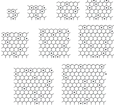
Fig. 2. Square distinct difference configurations with the largest number of dots possible forr= 2,3, . . . ,11.
Fig. 3. Hexagonal distinct difference configurations with the largest number of dots possible forr= 2,3, . . . ,10.
C. Small parameters
For small values ofr, we used a computer search to find a DD(m, r)withmas large as possible. The search shows that forr= 2,3, the largest suchm are 3 and 4 respectively, and for46r611the largest possiblemisr+ 2. Fig. 2 contains examples of configurations meeting those bounds.
Similarly, we found the best configurations DD∗(m, r) in the hexagonal grid (see Figure 3) for26r610.
III. ANTICODES ANDDDCS
(a) (b) (c)
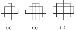
Fig. 4. Maximal anticodes in the square grid
anticode S of diameter r is said to be maximal if {x} ∪ S has diameter greater than r for any x /∈ S. Anticodes are important structures in various aspects of coding theory and extremal combinatorics [1]–[3], [13], [18], [33], [41].
The following two results provide an obvious connection between DDCs and anticodes.
Lemma 1. Any anticode S of diameter r is contained in a maximal anticodeS′of diameterr.
Corollary 2.ADD(m, r)is contained in a maximal anticode of (Euclidean) diameter r. The same statement holds for a
DD(m, r), DD∗(m, r) or DD∗(m, r) when the appropriate distance measure is used.
A. Maximal anticodes in the square grid
We start by defining three shapes in the square grid. We will prove that these shapes are the only maximal anticodes in the square grid when we use Manhattan distance.
ALee sphere of radius R is the shape in the square model which consists of one point as centre and all positions of Manhattan distance at most R from this centre. The area of this Lee sphere is2R2+ 2R+ 1. For the seminal paper on Lee
spheres see [27]. Figure 4a illustrates a Lee sphere of radius 2.
Abicentred Lee sphereof radius R is the shape in the square model which consists of two centre points (a2×1or an1×2 rectangle) and all positions of Manhattan distance at mostR from at least one point of this centre. The area of this bicentred Lee sphere is 2R2+ 4R+ 2. These shapes were used for
two-dimensional burst-correction in [8]. Figure 4b illustrates a bicentred Lee sphere of radius 2.
A quadricentred Lee sphere of radius R is the shape in the square model which consists of four centre points (a 2×2 square) and all positions of Manhattan distance at most R −1 from at least one point of this centre. The area of this quadricentred Lee sphere is 2R2 + 2R. These shapes
were defined using the name ‘generalized Lee sphere’ in [17]. Figure 4c illustrates a quadricentred Lee sphere of radius 3.
Theorem 3.
• For evenrthere are two different types of maximal
anti-codes of diameterrin square grid: the Lee sphere of radius
r
2 and the quadricentred Lee sphere of radius
r
2.
• For oddrthere is exactly one type of maximal anticode of
diameterrin the square grid: the bicentred Lee sphere of radiusr−21.
Proof: Let A be a maximal anticode of diameter r in the square grid.
Assume first that r is even, so r= 2ρ. We will embed A in the two-dimensional square grid in such a way that there is position inAon the liney=x, but no position below it. The Manhattan distance between a point on the line y = x+ 2ρ and a point on the line y =xis at least 2ρ and henceA is bounded by the linesy=xandy=x+2ρ. Similarly, without loss of generality we can assume that there is a position inA on the liney =−xory=−x+ 1and no position below this line, soAis bounded by the linesy=−xandy=−x+ 2ρ, or by the linesy=−x+ 1andy =−x+ 2ρ+ 1. These four lines define a Lee sphere of radiusρ or a quadricentred Lee sphere of radiusρ.
Now, assume that ris odd, sor= 2ρ+ 1. We will embed Ain the two-dimensional square grid in a way that a position of A lies on the line y = x, but no position lies below it. The Manhattan distance between a point on the liney=x+ 2ρ+ 1 and a point on the liney =x is at least2ρ+ 1 and henceAis bounded by the lines y=xandy =x+ 2ρ+ 1. Similarly, without loss of generality we can assume that there is a position of A on the line y =−x ory = −x+ 1 and no position below this line, and soAis bounded by the lines y =−xand y =−x+ 2ρ+ 1 or by the linesy = −x+ 1 andy=−x+ 2ρ+ 2. In either case, these four lines define a bicentred Lee sphere of radiusρ.
Finally, the following theorem is interesting from a theoret-ical point of view.
Theorem 4.There exists aDD(m, r)for which the only max-imal anticode of diameter r containing it is a Lee sphere (bicentred Lee sphere, quadricentred Lee sphere) of diameter
r.
Proof: We provide the configurations that are needed. All the claims in the proof below are readily verified and left to the reader.
When r is odd, we may take two points on the same horizontal line such that d(x, y) = r: this pair of points is in a bicentred Lee sphere of radius r−21. Whenr is even, the same example is contained in a Lee sphere of radiusr/2, but is not contained in a quadricentred Lee sphere of radiusr/2. Let r be even, and set R = r/2. The points (0, R−1), (0, R),(2R−2,0),(2R−2,2R−1), and(2R−1, R)form DD(5,2R). This set of points is not contained in a Lee sphere of radiusR, but is contained in a quadricentred Lee sphere of radiusR.
B. Maximal anticodes in the hexagonal grid
Theorem 5.There are exactly⌈r+1
2 ⌉different types of
maxi-mal anticodes of diameterrin the hexagonal grid, namely the anticodesA0,A1, . . . ,A⌈r−1
i be defined by the property that the linesy=x−icontains a point of A, but no point ofAlies below this line.
We claim thati>0. To see this, assume for a contradiction that i <0. Then A is contained in the region ofB bounded by the lines y = x−i, y = r, and x = 0. But the point (0, r+ 1)outsideBis within distancerfrom all the points of this region, contradicting the fact thatAis a maximal anticode. Thus,i>0 and our claim follows.
All the points on the line y = x−i that are inside B are within hexagonal distance r from all points on the lines y=x−i+j,06j6r, that lie insideB. All the points on the line y =x−i inside B have hexagonal distance greater thanrfrom all the points on the liney=x−i+r+ 1. Hence, as Ais maximal,Aconsists of all the points bounded by the linesy=x−iandy=x−i+rinsideB. It is easy to verify that each one of the r+ 1anticodesAi defined in this way is a maximal anticode. One can readily verify thatAiandAr−i are equivalent anticodes, since Ar−i is obtained by rotating Ai by 180 degrees. So the theorem follows.
Theorem 6.Letibe fixed, where06i6⌈r−21⌉. There exists aDD∗(m, r)for which the only maximal anticode of diameter
rcontaining it is of the formAi.
Proof: Again, we provide the configurations, and leave the verification of the details to the reader.
For each i, 1 6 i 6 r−21, Ai has six corner points. If we assign a dot to each corner point then we will obtain a DDC which cannot be inscribed in another maximal anticode. When r= 2R these six points do not define a DDC in AR. In this case we assign seven dots to AR as follows. In four consecutive corner points we assign a dot; in the next corner point we assign two dots in the adjacent points on the boundary ofAR; in the last corner point we assign a dot in the adjacent point on the boundary of AR towards the first corner point. When i= 0,Ai is a triangle and has three corner points. If we assign a dot to each of these corner points we will obtain a DDC which cannot be inscribed in another maximal anticode.
We now consider some basic properties of these ⌈r+12 ⌉
anticodes. First, the number of grid points in Ai is (r+ 1)2− i(i+1)
2 −
(r−i)(r+1−i)
2 =
(r+1)(r+2)
2 +i(r −i). The
smallest anticode is A0, an isosceles right triangle with base
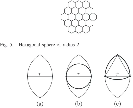
and height of length r+ 1containing (r+1)(2r+2) points. The largest anticode is thehexagonal sphereA⌈r−1
2 ⌉ of radiusr/2.
The hexagonal sphere contains 3(r+1)
2
4 points whenris odd,
and contains 3r2+64r+4 = 3 r
2
2
+ 3 r
2
+ 1 points when r is even. The hexagonal sphere of radius R is the shape in the hexagonal model which consists of a centre point and all positions in hexagonal distance at most R from this centre (Fig. 5).
C. Maximal anticodes with Euclidean distance
It seems much more difficult to classify the maximal an-ticodes in the square and hexagonal grids when we use Eu-clidean distance. Note that the representation of the hexagonal grid in the square grid does not preserve Euclidean distances,
Fig. 5. Hexagonal sphere of radius 2
r r r
(a) (b) (c)
Fig. 6. Anticodes in the Euclidean distance
and so we cannot use the map ξ. We expect that the overall shape of a maximal anticode in both models should be similar, since a maximal anticode in both models is just the intersection of a maximal anticode inR2with the centres of our squares or hexagons respectively. But the ‘local’ structure of an anticode will be different: for example, in the hexagonal grid we can have three dots that are pairwise at distancer, but this is not possible in the square grid.
Because maximal anticodes in R2 determine the shape of maximal anticodes in the square or hexagonal models, we conclude this section with a brief description of such anticodes.
An anticode is confined to the area as depicted in Figure 6a, where dots are two elements in the anticode at distance r. The most obvious maximal anticode is a circle of diameterr depicted in Figure 6b. Another maximal anticode is depicted in Figure 6c, and is constructed by taking three dots at the vertices of an equilateral triangle of sider, and intersecting the circles of radius rabout these dots. Between the ‘triangular’ anticode and the circle there are infinitely many other max-imal anticodes. We will need the following ‘isoperimetrical’ theorem; see Littlewood [32, Page 32] for a proof.
Theorem 7.LetAbe a region ofR2of diameterrand areaa. Thena6(π/4)r2.
We remark that the example of a circle of diameterrshows that the bound of this theorem is tight.
IV. UPPER BOUNDS ON THENUMBER OFDOTS
In this section we will provide asymptotic upper bounds on the number of dots that can be contained in a DDC, using a technique due to Tur´an [14], [15]. We start by considering upper bounds on the numbermof dots in a DD(m, r)and a DD∗(m, r), and then consider upper bounds in a DD(m, r) andDD∗(m, r). The results for small parameters in Section II might suggest that aDD(m, r)can always containr+ 2dots: our result (Theorem 9) that m 6 √1
2r+o(r) surprised us.
related to distance measures: we end the section with a brief discussion of this general situation.
A. Manhattan and hexagonal distances
Lemma 8.Letrbe a non-negative integer. LetAbe an anticode of Manhattan diameterrin the square grid. Letℓbe a positive integer such thatℓ6r, and letwbe the number of Lee spheres of radiusℓthat intersectAnon-trivially. Thenw612(r+2ℓ)2+
O(r).
Proof: LetA′ be the set of centres of the Lee spheres we are considering, so w = |A′|. We claim that A′ is an anticode of diameter at mostr+ 2ℓ. To see this, letc, c′∈ A′. Since the spheres of radiusℓ aboutc andc′ intersectA non-trivially, there exist elements a, a′ ∈ A such thatd(c, a)6ℓ andd(c′, a′)6ℓ. But then
d(c, c′)6d(c, a) +d(a, a′) +d(a′, c′)6ℓ+r+ℓ=r+ 2ℓ,
and so our claim follows.
LetA′′be a maximal anticode of diameterr+2ℓcontaining A′. Theorem 3 implies that A′′ is a Lee sphere, bicentred Lee sphere or quadricentred Lee sphere of radius R, where R=⌊(r+ 2ℓ)/2⌊. In all three cases, |A′′|= 2R2+O(R) =
Theorem 9.If aDD(m, r)exists, then
m6√1
2r+ (3/2
4/3)r2/3+O(r1/3).
Proof: We begin by giving a simple argument that leads to a linear bound onmin terms ofr, with an inferior leading term to the bound in the statement of the theorem. There are 2r2+2rnon-zero vectors of Manhattan lengthror less, where
a vector is a line with direction which connects two points. The distinct difference property implies that each such vector arises at most once as the vector difference of a pair of dots. Since a configuration ofmdots gives rise tom(m−1)vector differences, we find that
m(m−1)62r2+ 2r.
In particular, we see thatm6√2r+o(r) =O(r).
We now establish the bound of the theorem. Since all the dots are at distance at mostr, we see that all dots are contained in a fixed anticode A of the square grid of diameter r. Set ℓ = ⌊αr2/3⌋, where we will choose the constant α later so
as to optimize our bound. We cover A with all the ‘small’ Lee spheres of radius ℓ that intersect A nontrivially. Every point ofAis contained in exactlyasmall Lee spheres, where a = 2ℓ2+ 2ℓ+ 1. Moreover, by Lemma 8, we have used w
small Lee spheres, wherew6 12(r+ 2ℓ)2+O(r).
Let mi be the number of dots in the ith small Lee sphere. Let µ be the mean of the integers mi. Since every dot is contained in exactly a small Lee spheres, µ = am/w. We aim to show that
The first inequality in (1) follows from expanding the non-negative sumPwi=1(µ−mi)2, so it remains to show the second inequality.
The sum Pwi=1mi(mi −1) counts the number of pairs (L, d) where L is a small Lee sphere and d is a vector difference between two dots in ℓ. Every difference d arises from a unique ordered pair of dots in A, since the dots form a distinct difference configuration. Thus
where we sum over all non-zero vector differencesdand where k(d)is the number of Lee spheres of radiusℓthat contain any fixed pair of dots with vector differenced. If we assume that the first element of the pair of dots with vector difference d lies at the origin, we see that
X
d
k(d) =a(a−1)
since there are exactlyaLee spheres of radiusℓcontaining the origin, and each such sphere contributes1tok(d)for exactly a−1 values ofd. Thus we have established (1).
Now, the inequality (1) together with the fact that µ = am/w imply that
combine with (2) to show that
m6 √1
We now look at the hexagonal grid.
be a positive integer such thatℓ 6r, and letwbe the number of hexagonal spheres of radiusℓthat intersectAnon-trivially. Thenw6 34(r+ 2ℓ)2+O(r).
Proof: The set of centres of the hexagonal spheres of radiusℓthat have non-trivial intersection withAclearly form an anticode of diameter at mostr+ 2ℓ. Therefore the number w of such spheres is bounded by the maximal size of such an anticode. The results on the maximal anticodes in the hexagonal metric in Section III imply that
w6 14(3(r+ 2ℓ)2+ 6(r+ 2ℓ) + 4) = 34(r+ 2ℓ)2+O(r),
as required.
Theorem 11.If aDD∗(m, r)exists, then
m6 √
3 2 r+ (3
4/32−5/3)r2/3+O(r1/3).
Proof: The dots in a DD∗(m, r) form an anticode of diameter r. Letℓ =⌊2−2/33−1/6r2/3⌋. We may cover these
dots with the w hexagonal spheres of radius ℓ that contain one or more of these dots. By Lemma 10, we have that w6
3
4(r+ 2ℓ)2+O(r).
Using the fact that a hexagonal sphere of radiusℓcontains a points in the hexagonal grid, wherea= 3ℓ2+ 3ℓ+ 1, we may
argue exactly as in Theorem 9 to produce the bound (2). There are O(r2) vectors in the hexagonal grid of hexagonal length
ror less, so the argument in the first paragraph of Theorem 9 shows thatm=O(r). Sincem/a=O(r−1/3), the bound (2)
implies that
m6√w+O(r2/3) = √
3
2 r+O(r
2/3).
This bound on m implies that m/a = 21/33−1/6r−1/3 +
O(r−2/3), and so applying (2) once more we obtain the bound
of the theorem, as required.
One consequence of Theorem 11 is an answer to the ninth question asked by Golomb and Taylor [26]: ahoneycomb array
of orderR is a DDC whose shape is an hexagonal sphere of radiusR, and it contains2R+ 1dots (a dot in each hexagonal row, which makes this DDC akin to the Costas array). Do honeycomb arrays exist for infinitely many R? The conjecture in [26] is that the answer is YES. However, the answer is in fact NO, as the following corollary to Theorem 11 shows.
Corollary 12.Honeycomb arrays exist for only a finite number of values ofR.
Proof: A hexagonal sphere of radius R has diameter at most 2R (using hexagonal distance). Hence a honeycomb array is a DD∗(m,2R)with m= 2R+ 1. But Theorem 11 shows thatm6√3R+O(R2/3)and so no honeycomb array
exists whenR is sufficiently large.
In fact, numerical computations indicate that no honeycomb arrays exist for R > 644: for R in this range, there is a suitable choice of ℓsuch that a honeycomb array violates the inequality (2).
B. Euclidean distance
We now turn our attention to Euclidean distance. Our first lemma is closely related to Gauss’s circle problem:
Lemma 13. Let ℓ be a positive integer, and let S be a (Eu-clidean) circle of radius ℓ in the plane. Then the number of points of the square grid contained inSisπℓ2+O(ℓ).
Proof: Let c be the centre of S. Let X be the set of points of the square grid contained inS. DefineX to be the union of all unit squares whose centres lie in X. Clearly X has area|X|. The maximum distance from the centre of a unit square to any point in the unit square is at most1/√2, and so X is contained in the circle of radiusℓ+ (1/√2) with centre c. Similarly, every point in a circle of radiusℓ−(1/√2)with centrecis contained in X. Hence
π(ℓ−(1/√2))26|X|6π(ℓ+ (1/√2))2,
and so the lemma follows.
Lemma 14. Let r be a non-negative integer. Let A be an anticode in the square grid of Euclidean diameterr. Letℓ be a positive integer such thatℓ 6r, and letwbe the number of circles of radiusℓwhose centres lie in the square grid and that intersectAnon-trivially. Thenw6(π/4)(r+ 2ℓ)2+O(r).
Proof: As in Lemma 8, it is not difficult to see that the set A′of centres of circles we are considering form an anticode in the square grid of diameter at mostr+2ℓ. Note thatw=|A′|. LetX be the union of the unit squares whose centres lie inA′, so X has areaw. The maximum distance between the centre of a unit square and any other point in this square is1/√2, and soX is an anticode inR2of diameter at mostr+2ℓ+(1/√2). Hence, by Theorem 7,w6(π/4)(r+ 2ℓ+ (1/√2))2 and the lemma follows.
Theorem 15.If aDD(m, r)exists, then
m6 √π
2 r+ 3π1/3
25/3 r
2/3+O(r1/3).
Proof: The proof is essentially the same as the proof of Theorem 11, using Lemma 13 to bound the numbera of points in a sphere of radius ℓ, and using Lemma 14 instead of Lemma 10. The bound of the theorem is obtained if we set ℓ=⌊1/(22/3π1/6)r2/3⌋.
Lemma 16. Let ℓ be a positive integer, and let S be a (Eu-clidean) circle of radius ℓ in the plane. Then the number of points of the hexagonal grid contained in S is (2π/√3)ℓ2+
O(ℓ).
Proof: The proof of the lemma is essentially the same as the proof of Lemma 13. The hexagons whose centres form the hexagonal grid have area √3/2, and the maximum distance of the centre of a hexagon to any point in the hexagon is 1/√3. DefineX to be the set of points of the hexagonal grid contained inS, and letX be the union of all hexagons in our grid whose centres lie inX. ClearlyX has area(√3/2)|X|. The argument of Lemma 13 shows that
and so the lemma follows.
Lemma 17. Let r be a non-negative integer. Let A be an anticode in the square grid of Euclidean diameterr. Letℓ be a positive integer such thatℓ 6r, and letwbe the number of circles of radiusℓwhose centres lie in the hexagonal grid and that intersectAnon-trivially. Thenw6(π/(2√3))(r+ 2ℓ)2+
O(r).
Proof: The proof of this lemma is essentially the same as the proof of Lemma 14. The argument there with appropriate modifications shows that(√3/2)w6(π/4)(r+2ℓ+(1/√3))2
(where the factor of √3/2 comes from the fact that the hexagons associated with our grid have area √3/2).
Theorem 18.If aDD∗(m, r)exists, then
m6 √
π √
2 31/4r+
35/6
π1/3
24/3 r
2/3+O(r1/3).
Proof: The proof is the same as the proof of Theorem 15, using Lemmas 16 and 17 in place of Lemmas 13 and 14, and defining ℓ=⌊31/122−5/6π−1/6r2/3⌋.
C. More general shapes
All the theorems above consider a maximal anticode in some metric, and cover this region with small circles of radius ℓ. We comment (for use later) that the same techniques work for any ‘sensible’ shape that is not necessarily an anticode. (We just need that the number of small circles that intersect our shape is approximately equal to the number of grid points contained in the shape.) So we can prove similar theorems for DDCs that are restricted to lie inside regular polygons, for example. The maximal number of dots in such a DDC is at most √s+o(√s) when the shape contains s points of the grid.
V. PERIODICTWO-DIMENSIONALCONFIGURATIONS
The previously known constructions for DDCs restrict dots to lie in a line or a rectangular region (often a square region) of the plane. The application described in [6] instead demands that the dots lie in some anticode. The most straightforward approach to constructing DDCs for our application is to find a large square or rectangular subregion of our anticode, and use one of these known constructions to place dots in this subregion. This approach provides a lower bound for m that is linear in r, but in fact we are able to do much better than this by modifying known constructions (in the case of Robinson’s folding technique below) and by making use of certain periodicity properties of infinite arrays related to rectangular constructions. We will explain how this can be done in the next section. In this section we will survey some of the known constructions for rectangular DDCs, extend these constructions to infinite periodic arrays, and prove the properties we need for Section VI.
Let A be a (generally infinite) array of dots in the square grid, and let η and κbe positive integers. We say that A is
doubly periodicwith period(η, κ)ifA(i, j) =A(i+η, j)and A(i, j) = A(i, j+κ)for all integers i andj. We define the
density ofAto bed/(ηκ), wheredis the number of dots in anyκ×η sub-array ofA. Note that the period(η, κ)will not be unique, but that the density ofA does not depend on the period we choose. We say that a doubly periodic array Aof dots isa doubly periodicn×kDDCif everyn×ksub-array of A is a DDC. See [16], [34], [43] for some information on doubly periodic arrays in this context. We aim to present several constructions of doubly periodic DDCs of high density.
A. Constructions from Costas Arrays
A Costas arrayof order n is an n×n permutation array which is also a DDC. Essentially two constructions for Costas arrays are known, and both give rise to doubly periodic DDCs.
The Periodic Welch Construction:
Letαbe a primitive root modulo a primepand letAbe the square grid. For any integersiandj, there is a dot inA(i, j) if and only ifαi≡j (mod p).
The following theorem is easy to prove. A proof which also mentions some other properties of the construction is given in [7].
Theorem 19. Let A be the array of dots from the Periodic Welch Construction. ThenAis a doubly periodicp×(p−1)
DDC with period(p−1, p)and density1/p.
Indeed, it is not difficult to show that each p×(p−1) sub-array is a DDC with p−1 dots: a dot in each column and exactly one empty row. The(p−1)×(p−1)sub-array with lower left corner atA(1,1) is a Costas array.
The Periodic Golomb Construction:
Letα andβ be two primitive elements in GF(q), whereq is a prime power. For any integersi andj, there is a dot in A(i, j)if and only ifαi+βj= 1.
The following theorem is proved similarly to the proof in [7], [23].
Theorem 20. Let A be the array of dots from the Periodic Golomb Construction. ThenAis a doubly periodic(q−1)×(q− 1)DDC with period(q−1, q−1)and density(q−2)/(q−1)2.
Indeed, each(q−1)×(q−1)sub-array ofAis a DDC with q−2 dots; exactly one row and one column are empty. The (q−2)×(q−2) sub-array with lower left corner atA(1,1) is a Costas array.
If we take α = β in the Golomb construction, then the construction is known as the Lempel Construction. There are various variants for these two constructions resulting in Costas arrays with orders slightly smaller (by 1, 2, 3, or 4) or larger by one than the orders of these two constructions (see [24], [26]). These are of less interest in our discussion, as they do not extend to doubly periodic arrays in an obvious way.
B. Constructions from Golomb rectangles
Folded Ruler Construction:
Let S = {a1, a2,· · · , am} ⊆ {0,1, . . . , n} be a Golomb ruler of lengthn. Letℓandkbe integers such thatℓ·k6n+1. DefineAto be the ℓ×karray whereA(i, j),06i6k−1, 06j6ℓ−1, has a dot if and only ifi·ℓ+j=atfor some t.
Theorem 21.The arrayAof the Folded Ruler Construction is anℓ×kGolomb rectangle.
We now show how to adapt the Folded Ruler Construction to obtain a doubly periodicℓ×kDDC. We require a stronger object than a Golomb ruler as the basis for our folding construction, defined as follows.
Definition 5. Let A be an abelian group, and let D = {a1, a2, . . . , am} ⊆ Abe a sequence of m distinct elements
ofA. We say thatD is a B2-sequence over Aif all the sums
ai1+ai2 with16i16i26mare distinct.
For a survey onB2-sequences and their generalizations the
reader is referred to [35]. The following lemma is well known and can be readily verified.
Lemma 22. A subset D = {a1, a2, . . . , am} ⊆ A is a B2
-sequence overAif and only if all the differencesai1−ai2 with
16i16=i26mare distinct inA.
So, in particular, a Golomb ruler is exactly a B2-sequence
over Z. Note that a B2-sequence {a1, a2, . . . , am} over Zn produces a Golomb ruler{b1, b2, . . . , bm}whenever thebi are integers such that ai ≡ bi modn. Also note that ifD is a B2-sequence overZn anda∈Zn, then so is the shifta+D= {a+d: d∈D}. The following theorem, due to Bose [10], shows that largeB2-sequences overZn exist for many values ofn.
Theorem 23.Letqbe a prime power. Then there exists aB2
-sequencea1, a2, . . . , amoverZnwheren=q2−1andm=q. The Doubly Periodic Folding Construction:
Letnbe a positive integer andD={a1, a2, . . . , am}be a B2-sequence inZn. Letℓandkbe integers such thatℓ·k6n.
LetA be the square grid. For any integersiandj, there is a dot in A(i, j)if and only if at≡i·ℓ+j (mod n)for some t.
Theorem 24.LetAbe the array of the Doubly Periodic Folding Construction. ThenAis a doubly periodicℓ×kDDC of period
(g.c.d.n(n,ℓ), n)and densitym/n.
Proof: Letf(x, y) =x·ℓ+y. The period ofAfollows from the observation that for each two integers α andβ we havef(i, j) =f(i+α n
g.c.d.(n,ℓ), j+βn)≡i·ℓ+j (mod n).
The density of A is m/nfollows since there are exactly m dots in any nconsecutive positions in any column.
Let S be an ℓ×k sub-array, whose lower left-hand corner is atA(i, j). An alternative construction of the dots inS is as follows. Take the shift(i·ℓ+j)+DofD, which is also aB2
-sequence in Zn. Let D′ be the corresponding Golomb ruler
in {0,1, . . . , n−1}, so a∈ D if and only if a≡bmodn, whereb∈(i·ℓ+j) +D. Then form dots in S by using the Folded Ruler Construction. Hence, by Theorem 21, the dots inS form a DDC and so the theorem follows.
The following slightly different construction also produces doubly periodic Golomb rectangles.
The Chinese Remainder Theorem Construction:
Let n be a positive integer and let D ={a1, a2, . . . , am} be aB2-sequence in Zn. Letn=ℓ·kbe any factorization of nsuch thatg.c.d.(ℓ, k) = 1. For any two integersiandj we place a dot inA(i, j), if and only ifat= (i·ℓ+j·k) (mod n) for somet.
Theorem 25. Let Abe the array constructed by the Chinese Remainder Theorem construction. ThenAis a doubly periodic
ℓ×kDDC of period(k, ℓ)and densitym/n. Moreover, every
ℓ×ksub-array ofAcontains exactlymdots.
Proof: Letf(x, y) =x·ℓ+y·k. For any two integersα andβwe havef(i, j)≡f(i+αk, j+βℓ)≡i·ℓ+j·k(mod n). So the definition ofAimplies thatAis doubly periodic with period(k, ℓ).
Since ℓ and k are relatively primes, it follows (from the Chinese Remainder Theorem) that each integersin the range 06s6ℓ·k−1, has a unique representation ass=d·ℓ+e·k, where06d6k−1,06e6ℓ−1. Hence everyℓ×k sub-array ofAhasmdots corresponding to themelements of the B2-sequenceD. In particular, this implies thatAhas density
m/n.
Assume for a contradiction that there exists an ℓ×k sub-arrayS ofAthat is not a DDC. Suppose that the lower left-hand corner of S is at A(i, j). The distribution of dots in S is the same as the distribution in the sub-array with lower left-hand corner the origin once we replace D by the shift (iℓ+jℓ) +D. So, without loss of generality, we may assume that the lower left-hand corner of S lies at the origin. As the distinct difference property fails to be satisfied, there are four positions with dots inAof the form:
A(i1, j1) A(i1+d, j1+e)
A(i2, j2) A(i2+d, j2+e)
where i1, i1+d, i2, i2+d ∈ {0,1, . . . , k−1} and j1, j1+
e, j2, j2+e ∈ {0,1, . . . , ℓ−1}. By the definition of A we
have
(i1+d)ℓ+ (j1+e)k−(i1ℓ+j1k) =d·ℓ+e·k
(i2+d)ℓ+ (j2+e)k−(i2ℓ+j2k) =d·ℓ+e·k
Since by Lemma 22 each nonzero residuesmodulonhas at most one representation as a difference from two elements of D, it follows that the pairs
{A(i1, j1),A(i1+d, j1+e)}
{A(i2, j2),A(i2+d, j2+e)}
VI. LOWER BOUNDS
A. Manhattan distance
In this section we will prove that there exists a DD(m, r) with √r
2 −o(r) dots: this attains asymptotically the upper
bound of Theorem 9. We will see that this construction is actually using folding in a slightly different way. We further show that we can construct a doubly periodic array in which each Lee sphere of diameterris a DDC with √r
2+o(r)dots.
The LeeDD Construction:
Let r be an integer, and define R = ⌊r2⌋. Let D =
{a1, a2, . . . , aµ} be a ruler of length n. Define f(i, j) = iR+j(R+ 1) +R2+R. LetAbe the Lee sphere of radiusR
centred at (0,0), so Ahas the entry A(i, j) if|i|+|j|6R. We place a dot in A(i, j)if and only iff(i, j)∈D.
Theorem 26.The Lee sphereAof the LeeDD Construction is aDD(m, r), wherem=D∩ {0,1, . . . ,2R2+ 2R}.
Proof: We first note that if|i|+|j|6Rthen the smallest value that the function f takes is 0 and the largest value is 2R2+ 2R. Next, we claim that if(i
1, j1)and(i2, j2)are two
distinct points such that |i1|+|j1| 6 |i2|+|j2| 6 R then
f(i1, j1) 6= f(i2, j2). Assume the contrary, that f(i1, j1) =
f(i2, j2). Soi1R+j1(R+ 1) +R2+R=i2R+j2(R+ 1) +
R2+Rand therefore(i
2−i1)R= (j1−j2)(R+1). Ifi1=i2,
thenj1=j2which contradicts our assumption that(i1, j1)and
(i2, j2)are distinct. So we may assume thati16=i2. Similarly,
we may assume that j1 6= j2. The equality (i2 −i1)R =
(j1−j2)(R+ 1)now implies thatR+ 1divides|i2−i1|and
Rdivides|j2−j1|. This implies that|i2−i1|+|j2−j1|>2R,
but
|i2−i1|+|j2−j1|6|i1|+|j1|+|i2|+|j2|62R,
and so we have a contradiction. Thus, f(i1, j1) 6=f(i2, j2).
This implies that each one of the integers between 0 and 2R2+ 2R is the image of exactly one pair (i, j). In
partic-ular, the number m of dots in the configuration is exactly
D∩ {0,1, . . . ,2R2+ 2R}.
Since A is a Lee sphere of radius R, it follows that the Manhattan distance between any two points is at most2R6r. Now, assume for a contradiction thatAis not aDD(m, r), so there exist four positions with dots in Aas follows:
A(i1, j1) A(i1+d, j1+e)
A(i2, j2) A(i2+d, j2+e)
By definition we have that
f(i1, j1), f(i1+d, j1+e), f(i2, j2), f(i2+d, j2+e)∈D.
But then f(i1+d, j1+e)−f(i1, j1) =f(i1+d, j1+e)−
f(i1, j1) =dR+e(R+ 1), contradicting the fact thatD is a
ruler.
Thus, the Lee sphere A of the LeeDD Construction is a DD(m, r).
Corollary 27 There exists aDD(m, r)in which m = √r
2 −
o(r).
24 17 20 23 10 13 16 19 22 3 6 9 12 15 18 21
2 5 8 11 14 1 4 7
0
Fig. 7. Folding along diagonals
Proof: Define R =⌊r/2⌋ and letn = 2R2+ 2R+ 1.
There exists a ruler of length at most n containing m dots, where m > √n+o(√n): see [4], [30], [40]. Let D ⊆ {0,1, . . . , n−1} be such a ruler. The corollary now follows, by Theorem 26.
It is worth mentioning that the LeeDD Construction is actually a folding of the ruler by the diagonals of the Lee sphere. Figure 7 illustrates why this is the case, by labelling the positions in a Lee sphere of radius 3 by the values of f(i, j) at these positions. So if we use a B2-sequence over
Zn instead of a ruler in the LeeDD Construction we obtain a doubly periodic array with nice properties:
The Doubly Periodic LeeDD Construction:
Letrbe an integer,R=⌊r2⌋, and letD={a1, a2, . . . , aµ}
be a B2-sequence over Zn, where n > 2R2+ 2R+ 1. Let
f(i, j)≡iR+j(R+ 1) modn. LetAbe the square grid. For each two integersiandj, there is a dot inA(i, j)if and only iff(i, j)∈D.
Similarly to Theorem 26 we can prove the following result.
Theorem 28.The arrayAconstructed in the LeeDD Construc-tion is doubly periodic with period(n, n)and densityµ/n. The dots contained in any Lee sphere of radiusRform a DDC.
Proof: The first statement of the theorem is obvious. The second statement follows as in the proof of Theorem 26, once we observe that f is an injection when restricted to any Lee sphere of radiusR.
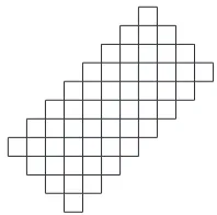
In Subsections VI-D and VI-E we will make use of an extension of this construction. For positive integersR andt, an(R, t)-diagonally extended Lee sphereis a set of positions in the square grid defined as follows. Let (i0, j0)∈ Z2, and
define C = {(i0+k, j0+k) : 0 6 k 6 t−1}. Then an
(R, t)-diagonally extended Lee sphere is the union of the Lee spheres of radiusRwith centres lying inC. (See Fig. 8 for an example.) An(R, t)-diagonally extended Lee sphere contains exactly2R2+t(2R+ 1)positions; the Lee sphere of radiusR
is the special case whent= 1. We observe that by choosing n>2R2+t(2R+ 1), we can generalize the doubly periodic
LeeDD construction by continuing folding along the diagonals of the rectangle. This yields the following corollary, which will prove useful in the construction of configurations for the hexagonal grid.
Fig. 8. A (3,5)-diagonally extended Lee sphere
using the doubly periodic LeeDD Construction. Then A is a doubly periodic array with densityµ/n. The dots contained in any(R,⌊aR⌋)-diagonally extended Lee sphere form a DDC. There exists a family ofB2sequences so thatAhas density at
least1/p(2 + 2a)R2+o(R2).
Proof: To establish the final statement of the corollary, we choose a family of B2 sequences as follows. Let p be
the smallest prime such that p2 −1 > (2 + 2a)R2 +aR,
and define n=p2−1. By Ingham’s classical result [29] on
the gaps between primes, we have that n 6 (2 + 2a)R2+
O(R13/8) = (2 + 2a)R2+o(R2). By Theorem 23, there exists
a B2 sequence overZn withµ=p. Hence the density ofA is
µ/n=p/(p2−1)>1/p(2 + 2a)R2+o(R2),
as required.
B. A General Technique
LetS be a shape (a set of positions) in the square grid. We are interested in finding large DDCs contained inS, where (for example)S is an anticode. This subsection presents a general technique for showing the existence of such DDCs, using the doubly periodic constructions from Section V.
We write (i, j) +S for the shifted copy{(i+i′, j+j′) : (i′, j′) ∈ S} of S. Let A be a doubly periodic array. We say thatAis a doubly periodicS-DDCif the dots contained in every shift (i, j) +S of S form a DDC. So the doubly periodic arrays constructed in Section V are all doubly periodic S-DDCs where S is a square or a rectangle; the arrays in Theorem 28 and Corollary 29 are doubly periodic S-DDCs with S a Lee sphere and diagonally extended Lee sphere respectively. The following lemma follows in a straightforward way from our definitions:
Lemma 30.LetAbe a doubly periodicS-DDC, and letS′ ⊆ S. ThenAis a doubly periodicS′-DDC.
We will use doubly periodic DDCs to prove the existence of the configurations we are most interested in, using the following theorem.
Theorem 31.LetSbe a shape, and letAbe a doubly periodic
S-DDC of densityδ. Then there exists a set of at least⌈δ|S|⌉
dots contained inSthat form a DDC.
Proof: Let the period of Abe(η, κ). Writemi,j for the number of dots of A contained in the shift (i, j) +S of S.
NowAis periodic, so the definition of the density ofAshows
that η
X
i=1
κ
X
j=1
mi,j= (ηκ)δ|S|.
Hence the average size of the integer mi,j is δ|S|, so there exists an integermi′,j′ such that mi′,j′ >⌈δ|S|⌉. Themi′,j′ dots in(i′, j′) +Sform a DDC, by our assumption onA, and so the appropriate shift of these dots provides a DDC in S with at least⌈δ|S|⌉ dots, as required.
C. Euclidean distance in the square model
This subsection illustrates our general technique in the square grid using Euclidean distance. So we wish to construct aDD(m, r)withm as large as possible.
LetR=⌊r/2⌉, and letS be the set of points in the square grid that are contained in the Euclidean circle of radius R about the origin. We construct a DDC contained in S with many dots: any such configuration is clearly aDD(m, r)for some value ofm. The most straightforward approach is to find a large square contained inS (which will have sides of length approximately √2R), and then add dots within this square using a Costas array. This will produce a DD(m, r)where
m=√2R−o(R) = √1
2r−o(r)≈0.707r.
To motivate our better construction, we proceed as follows. We find a square of sidenwheren >√2Rthat partially overlaps our circle: see Figure 9. The constructions of Section V show that there exist doubly periodicn×nDDCs that have density approximately1/n. So Theorem 31 shows that for any shape S′ within the square, there exist DDCs inS′ that have at least |S′|/ndots. LetS′ be the intersection of our square with S. Definingθas in the diagram, some basic geometry shows that the area ofS′ is
|S′|= (π/2)−2θ+ sin 2θ
2 cos2θ |S|= 2R
2((π/2)−2θ+ sin 2θ).
Since n = 2Rcosθ, Theorem 31 shows that the density of dots within S′ can be about 1/n= 1/(2Rcosθ) when n is large. So we can hope for at least µR dots, where µ is the maximum value of
((π/2)−2θ+ sin 2θ)/cosθ
on the interval 0 6θ 6π/4. In fact µ≈1.61589, achieved when θ ≈ 0.41586 (and so when n = rcosθ = cr, where c≈0.914769).
Theorem 32. Let µ be defined as above. There exists a
DD(m, r)in whichm= (µ/2)r−o(r)≈0.80795r.
Note that Theorem 15 gives an upper bound on m of the form m6(√π/2)r+o(r)≈0.88623r. Proof: Define c ≈ 0.91477 as above. Let q be the smallest prime power such that q > cr. We have thatcr < q < cr+ (cr)5/8, by a
classical result of Ingham [29] on the gaps between primes; so in particularq∼cr. By Theorem 20, there exists a doubly periodic(q−1)×(q−1)DDCAof density(q−2)/(q−1)2.
R θ
n
2
Fig. 9. Square intersecting a circle
| {z }
aR
R
Alr −1 2
m
Fig. 10. A diagonal rectangle intersecting the image of a hexagonal sphere
of radius⌊r/2⌋about the origin. ThenAis a doubly periodic S′-DDC. By Theorem 31, there exists a DDC in S′ with at least mdots, where |S′|(q−2)/(q−1)2. But the geometric
argument above shows that |S′|(q−2)/(q−1)2 ∼ (µ/2)r,
and so the theorem follows.
D. Hexagonal distance
By representing the hexagonal anticodes in the square grid, we may use Theorem 31 to show the existence of aDD∗(m, r) where mis large. The method of producing lower bounds is essentially the same as above, but the geometrical problem we are solving is different, with the images under ξ of the maximal anticodes Ai replacing the circle, and the DDC contained a diagonally extended Lee sphere of Corollary 29 replacing the Costas array contained in a square. Here we consider the case of configurations contained in the hexagonal sphere A⌈(r−1)/2⌉; the cases of the other anticodes may be handled in a similar fashion. The problem we are solving is pictured in Fig. 10. The figure shows the image under ξ of the hexagonal sphere of radius R = ⌊r/2⌋ in bold; the square of side 2R+ 1 containing this image is also shown. The hexagonal sphere contains a Lee sphere of radiusR with the same centre; the region S we consider is the (R,⌊aR⌋) -diagonally extended Lee sphere whose mid-point is at the centre of the hexagonal sphere: see Fig. 10. Let S′ be the intersection ofS with the image of the hexagonal sphere. We
2t
√2at
2t
√3t
t at
Fig. 11. A(t,⌊at⌋)-diagonally extended Lee sphere is transformed into a rotated square (whenat= (√3−1)t+ 1)
have that |S′|=R2(2 + 2a−a2) +o(R2). By Corollary 29,
there is a doubly periodic S-DDC of density at least 1/√n wheren= 2R2(1 +a) +o(R2). Thus Theorem 31 shows that
there is a DDC contained in S′ containing µR−o(R) dots, whereµis the maximum of
2 + 2a−a2
√
2√1 +a .
It can be seen that µ = 2 3
3 2 1+2√7
√
2+√7 ≈ 1.58887, achieved
whena= −1+3√7. SinceS′is contained in a hexagonal sphere of radius R, all pairs of dots in our DDC are at hexagonal distance at mostr. Thus we have the following theorem:
Theorem 33. Let µ be defined as above. There exists a
DD∗(m, r)in whichm= (µ/2)r−o(r)≈0.79444r.
E. Euclidean distance in the hexagonal model
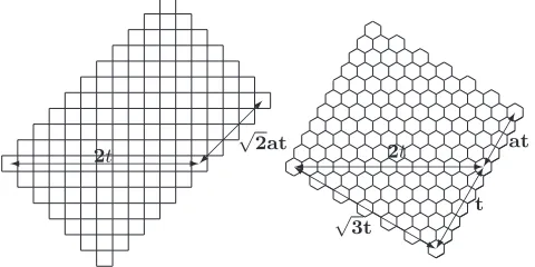
In this subsection we will obtain a construction for a DD∗(m, r) contained within a circle of radius R = ⌊r/2⌋, again based on the doubly periodic LeeDD construction. We first observe that a diagonally extended Lee sphere in the square grid is transformed by ξ−1 into a (rotated) rectangle
in the hexagonal grid. In particular, a (t,⌊(√3−1)t+ 1⌋) -diagonally extended Lee sphere is transformed by ξ−1 into a set of hexagons whose centres all lie within a (rotated) squareS of side√3t (see Fig. 11). Corollary 29 shows that there is a doubly periodicS-DDC with density1/√n, where n= 2√3t2+o(t2).
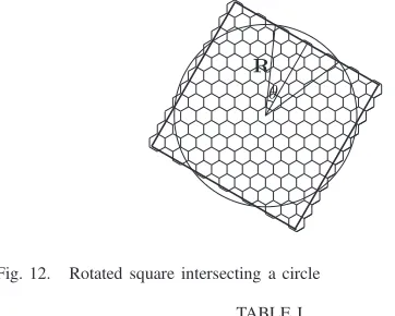
Consider (see Fig. 12) a circle of radiusR and a squareS of sideswheres= 2Rcosθ. Since a hexagon has area√3/2, the squareScontains(8/√3)R2cos2θ+O(R)hexagons. Let
S′ be the intersection of S with the circle of radius R. The calculations in Subsection VI-C show that
|S′|=(π/2−2θ+ sin 2θ)
2 cos2θ |S|+O(R).
The previous paragraph shows that there is an periodic S′ -DCC of densityδ= 1/√n, wheren= (2/√3)s2+o(s2). So
Theorem 31 now implies that there exists a distinct difference configuration inS′ containing at leastm dots, where
m=
q
2
√
3(π/2−2θ+ sin 2θ)
θ R
Fig. 12. Rotated square intersecting a circle
TABLE I
UPPER AND LOWER BOUNDS ON THE NUMBER OF DOTS IN A DISTINCT
DIFFERENCE CONFIGURATION
As in Subsection VI-C, we may takeθ≈0.41586to maximise this expression. Hence we have proved the following theorem:
Theorem 34. Letµ ≈ 1.61589be the constant defined above Theorem 32. There exists aDD∗(m,r)in which the number of dots is at leastq√2
3µR−o(R)≈0.86819r.
VII. CONCLUSION
We introduced the concept of a distinct difference config-uration and gave specific examples for both the square and hexagonal grids for small parameters. We went on to provide general constructions for such configurations, as well as upper and lower bounds on the maximum number of dots such configurations may contain. In the case of distinct difference configurations using Manhattan distance these bounds are tight asymptotically, as we have provided a construction for configurations which meets the leading term in our upper bound. For the remaining classes of configurations, there is a gap between the upper and lower bounds we have provided (see Table I). We believe the upper bounds to be realistic, and it is an interesting challenge to provide constructions that meet these bounds.
REFERENCES
[1] R. Ahlswede, H. K. Aydinian, and L. H. Khachatrian, “On perfect codes and related concepts,”Designs, Codes Crypto., vol. 22, pp. 221-237, 2001.
[2] R. Ahlswede and L. H. Khachatrian, “The complete nontrivial-intersection theorem for systems of finite sets,”J. Combin. Theory, Series A, vol. 76, pp. 121–138, 1996.
[3] R. Ahlswede and L. H. Khachatrian, “The diametric theorem in Ham-ming spaces–optimal anticodes,”Adv. Appl. Math., vol. 20, pp. 429–449, 1998.
[4] M. D. Atkinson, N. Santoro, and J. Urrutia, “Integer sets with distinct sums and differences and carrier frequency assignments for nonlinear re-peaters”,IEEE Transactions on Communications, vol. COM-34, pp. 614– 617, 1986.
[5] W. C. Babcock, “Intermodulation interference in radio systems,”Bull. Sys. Tech. Journal, pp. 63–73, June 1953.
[6] S. R. Blackburn, T. Etzion, K. M. Martin, and M. B. Paterson, “Efficient key predistribution for grid-based wireless sensor networks,” Lecture Notes in Computer Science, vol. 5155, pp. 54–69, August 2008. [7] S. R. Blackburn, T. Etzion, K. M. Martin, and M. B. Paterson, “Distinct
difference configurations: multihop paths and key predistribution in sensor networks”, preprint.
[8] M. Blaum, J. Bruck, and A. Vardy, “Interleaving schemes for mul-tidimensional cluster errors”, IEEE Trans. Inform. Theory, vol. IT-44, pp. 730–743, March 1998.
[9] A. Blokhuis and H. J. Tiersma, “Bounds for the size of radar arrays”, IEEE Trans. Inform. Theory, vol. IT-34, pp. 164–167, January 1988. [10] R. C. Bose, “An affine analogue of Singer’s theorem”,J. Indian Math.
Soc. (N.S.), vol. 6, pp. 1-15, 1942.
[11] J. H. Conway and N. J. A. Sloane, Sphere Packings, Lattices, and Groups,New York: Springer-Verlag, 1993.
[12] J. P. Costas, “Medium constraints on sonar design and performance,” in EASCON Conv. Rec., pp. 68A–68I, 1975.
[13] P. Delsarte, “An algebraic approach to association schemes of coding theory”,Philips J. Res., vol. 10, pp. 1–97, 1973.
[14] P. Erd˝os, R. Graham, I. Z. Ruzsa, and H. Taylor, “Bounds for arrays of dots with distinct slopes or lengths”,Combinatorica, vol. 12, pp. 39–44, 1992.
[15] P. Erd˝os and P. Tur´an, “On a problem of Sidon in additive number theory and some related problems”,J. London Math. Soc., vol. 16, pp. 212–215, 1941.
[16] T. Etzion, “Combinatorial designs derived from Costas arrays,” in Sequences, R. M. Capocelli editor, New York, NY: Springer Verlag, pp. 208–227, 1989.
[17] T. Etzion, “Tilings with generalized Lee spheres,” in Mathematical Properties of Sequences and Other Combinatorial Structures, J. S. No, H. Y. Song, T. Helleseth, and P. V. Kumar, editors, Kluwer Academic Publishers, pp. 181–198, 2003.
[18] T. Etzion, M. Schwartz, and A. Vardy, “Optimal tristance anticodes in certain graphs,”J. Combin. Theory, Series A, vol. 113, pp. 189–224, 2006.
[19] A. Freedman and N. Levanon, “Any twoN×N Costas signals must have at least one common ambiguity sidelobe ifN > 3– a proof”, Proceedings of the IEEE, vol. 73, pp. 1530–1531, October 1985. [20] R. Gagliardi, J. Robbins, and H. Taylor, “Acquisition sequences in PPM
communications”,IEEE Trans. Inform. Theory, vol. IT-33, pp. 738–744, September 1987.
[21] R. A. Games, “An algebraic construction of sonar sequences using M-sequences,”SIAM J. Algebraic and Discrete Methods, vol. 8, pp. 753– 761, October 1987.
[22] S. W. Golomb, “How to number a graph,” in Graph Theory and Computing, Academic press, pp. 23–37, 1972.
[23] S. W. Golomb, “Algebraic constructions for Costas arrays,”J. Combin. Theory, Series A, vol. 37, pp. 13–21, 1984.
[24] S. W. Golomb, “TheT4andG4constructions for Costas arrays”,IEEE
Trans. Inform. Theory, vol. IT-38, pp. 1404–1406, 1992.
[25] S. W. Golomb and H. Taylor, “Two-dimensional synchronization pat-terns for minimum ambiguity”,IEEE Trans. Inform. Theory, vol. IT-28, pp. 600–604, 1982.
[26] S. W. Golomb and H. Taylor “Constructions and properties of Costas arrays”,Proceedings of the IEEE, vol. 72, pp. 1143–1163, 1984. [27] S. W. Golomb and L. R. Welch, “Perfect codes in the Lee metric and
the packing of polyominos”,SIAM J. Appl. Math., vol. 18, pp. 302–317, 1970.
[28] J. Hamkins and K. Zeger, “Improved bounds on maximum size binary radar arrays”, IEEE Trans. Inform. Theory, vol. IT-43, pp. 997–1000, May 1997.
[29] A.E. Ingham, “On the difference between consecutive primes”,Quart. J. Math. Oxford (O.S.)vol. 8, pp. 255-266, 1937.
[30] A. W. Lam and D. V. Sarwate, “On optimum time-hopping patterns”, IEEE Transactions on Communications, vol. COM-36, pp. 380–382, 1988.
[31] H. Lefmann and T. Thiele, “Point sets with distinct distances”, Combi-natorica, vol. 15, pp. 379–408, 1995.
[32] J.E. Littlewood (B. Bollob´as, Ed),Littlewood’s miscellany, Cambridge University Press, Cambridge, 1986.
[33] W. J. Martin and X. J. Zhu, “Anticodes for the Grassman and bilinear forms graphs,”Designs, Codes, and Crypt., vol. 6, pp. 73–79, 1995. [34] O. Moreno, R. A. Games, and H. Taylor, “Sonar sequences from Costas
[35] K. O’Bryant, “A complete annotated bibliography of work related to Sidon sequences”, The Electronic Journal of Combinatorics, DS11, pp. 1–39, July 2004.
[36] R. E. Peile and H. Taylor, “Sets of points with pairwise distinct slopes”, Computers and Mathematics, vol. 39, pp. 109–115, 2000.
[37] J. P. Robinson “Golomb rectangles”, IEEE Trans. Inform. Theory, vol. IT-31, pp. 781–787, 1985.
[38] J. P. Robinson “Golomb rectangles as folded ruler”,IEEE Trans. Inform. Theory, vol. IT-43, pp. 290–293, 1997.
[39] J. P. Robinson “Genetic search for Golomb arrays”,IEEE Trans. Inform. Theory, vol. IT-46, pp. 1170–1173, 2000.
[40] J. P. Robinson and A. J. Bernstein “A class of binary recurrent codes with limited error propagation”,IEEE Trans. Inform. Theory, vol. IT-13, pp. 106–113, 1967.
[41] M. Schwartz, and T. Etzion, “Codes and anticodes in the Grassman graph,”J. Combin. Theory, Series A, vol. 97, pp. 27–42, 2002.
[42] J. B. Shearer, “Golomb rulers,”http://www.research.ibm.com/people/s/shearer/grule.html. [43] H. Taylor “Non-attacking rooks with distinct differences”,
Communica-tion Sciences Institute, University of Southern California, Tech. Report CSI-84-03-02, March 1984.
[44] Z. Zhang, “A note on arrays of dots with distinct slopes”,Combinatorica, vol. 13, pp. 127–128, 1993.