On
l
1
Mean and Variance Filtering
Bo Wahlberg, Cristian R. Rojas and Mariette Annergren
Automatic Control Lab and ACCESS, School of Electrical Engineering,
KTH Royal Institute of Technology, SE-100 44 Stockholm, Sweden.
Abstract— This paper addresses the problem of segmenting a time-series with respect to changes in the mean value or in the variance. The first case is when the time data is modeled as a sequence of independent and normal distributed random variables with unknown, possibly changing, mean value but fixed variance. The main assumption is that the mean value is piecewise constant in time, and the task is to estimate the change times and the mean values within the segments. The second case is when the mean value is constant, but the variance can change. The assumption is that the variance is piecewise constant in time, and we want to estimate change times and the variance values within the segments. To find solutions to these
problems, we will study anl1 regularized maximum likelihood
method, related to the fused lasso method andl1trend filtering,
where the parameters to be estimated are free to vary at each sample. To penalize variations in the estimated parameters, the
l1-norm of the time difference of the parameters is used as a
regularization term. This idea is closely related to total variation denoising. The main contribution is that a convex formulation of this variance estimation problem, where the parametrization is based on the inverse of the variance, can be formulated
as a certain l1 mean estimation problem. This implies that
results and methods for mean estimation can be applied to the challenging problem of variance segmentation/estimation.
Copyright 1998 IEEE. Published in the Proceedings of the 45th Annual Asilomar Conference on Signals, Systems, and Computers, November 6-9, 2011, Pacific Grove, California, USA Personal use of this material is permitted. However, permission to reprint/republish this material for advertising or promotional purposes or for creating new collective works for resale or redistribution to servers or lists, or to reuse any copyrighted component of this work in other works, must be obtained from the IEEE.
I. INTRODUCTION
The problem of estimating the mean, trends and variances in time series data is of fundamental importance in signal processing and in many other disciplines such as processing of financial and biological data. This is typically done to preprocess data before estimating for example parametric models. For non-stationary data it is also important to be able to detect changes in mean and variances and segment the data into stationary subsets. A classical way is to use windowing to handle time-variations, by for example subtracting the windowed sample mean estimate from the data or scaling
e-mails: [email protected], [email protected], [email protected].
This work was partially supported by the Swedish Research Council and the Linnaeus Center ACCESS at KTH. The research leading to these results has received funding from The European Research Council under the European Community’s Seventh Framework program (FP7 2007-2013) / ERC Grant Agrement N. 267381
the data with a windowed estimate of the variance. More advanced detection and segmentation methods are often based on probabilistic models, such as Markov models, and have a lot of tuning and user choices, [8]. An alternative way to approach this problem is to use regularization to penalize variations and changes in the estimated parameter vector. Recently, there has been a lot of efforts on applying l1-norm regularization in estimation in order to obtain convex
optimization problems, [9], [5]. Our work is inspired by the l1 trend filtering method in [10] and the fused lasso
method, [13]. Thel1trend filtering method considers changes
in the mean value of the data. Here we are also interested in changes in the variance. This problem is closely related to the covariance selection problem introduced in [4]. The paper [1] formulates this as a convex optimization problem by using the inverse of the covariance matrix as parameter, see also [10]. This idea is also used in the graphical lasso method, [6].
The paper is organized as follows. In Section II the general problem formulation is specified. Section III considers the special case of mean estimation, while Section IV deals with variance estimation and its relation to mean estimation. Sec-tion V contains a numerical example of variance estimaSec-tion, and Section VI discusses the extension to the multi-variate case. The paper is concluded in Section VII.
II. PROBLEMSTATEMENT
Consider the independent scalar sequence {yt} which satisfies
yt∼N (mt,σt2),
where both the mean {mt} and the variance {σ2
t} are (unknown) piecewise constant sequences. Assume that the measurements {y1 · · · yN} are available, and we are inter-ested in estimatingm1, . . . ,mN andσ12, . . . ,σN2.
To solve this problem, first notice that the model yt ∼
N(mt,σt) is a standard exponential family with canonical parameters, [3, Example 1.2],
µt:=mt/σt2∈R, ηt:=−1/2σt2∈R−
This means that the log-likelihood of {µ1, . . . ,µN,
η1, . . . ,ηN}given{y1 · · ·yN} is
l(µ1, . . . ,µN,η1, . . . ,ηN) =− N
2lnπ+ N
∑
t=1
ln(−ηt)
2
+µ
2
t 4ηt
+ηtyt2+µtyt
.
Moreover, by [3, Theorem 1.13] it follows that l is strictly concave on
{(µ1, . . . ,µN,η1, . . . ,ηN): µt∈R,ηt∈R−,t=1, . . . ,N}.
Assumption: The prior knowledge is that the sequences {mt} and{σ2
t} are piecewise constant in time. This means that the difference sequences {mt+1−mt} and{σt2+1−σt2} are sparse.
Inspired by [10] we propose an estimator based on the solution of the following optimization problem:
minimize
This a convex optimization problem where the cost function is separable, plus two terms that are separable in the dif-ference between consecutive variables. The l1-norm is used
to penalize non-sparse solutions, while still having a convex objective function. Standard software for convex optimiza-tion can be used to solve (1). However, it is possible to use the special structure to derive more efficient optimization algorithms for (1), see [2], [14].
III. MEANESTIMATION
Consider the problem of mean segmentation under the assumption that the variance is constant. The optimization problem (1) then simplifies to
minimize
Thet:th element of the sub-differential of the cost function equals
Fort=1 andt=N obvious modifications have to be done to take the initial and end conditions into account. Using the incremental structure of the sub-differential, it makes sense to add up the expressions(4) to obtain
k
This is more or less the sub-differential with respect to the variables r1=m1, rk =mk−mk−1, k=2, . . . ,N. For
optimality the sub-gradient should include zero, which leads to the optimality conditions
k
The "empirical mean"
b
obtained from (7), satisfies also the first N−1 optimality conditions (6) if
if λ1 is large enough. Since the optimization problem (2)
is convex, the sub-differential condition is necessary and sufficient. Hence we have now derived theλmax result, [10]
[λ1]max= max
obvious by diving (9) byk,
1
Hence, we compare the empirical means for the sequences of lengthk=1, . . . ,N−1 with m, and then relateb λ to the maximum deviation.
The λmax result is very useful in order to find a good
choice ofλ, and also to derive efficient numerical solvers.
IV. VARIANCEESTIMATION
We will now study the variance estimation problem under the assumption that the mean values are known. We can, without losing generality, assume thatmt=0. For this special case the optimization problem (1) equals
minimize
We will now show that (10) is equivalent, in the sense of having related optimal solution, to the optimization problem
where
which means that the sign of the differences is not affected by the transformation σ2
t =−1/(2ηt). This will be critical in deriving the equivalence result. The formulation (12) also makes sense from a practical point of view, since the variance of yt (in the zero mean case) is the mean of y2t. Notice, however, that this is not directly obvious from the log-likelihood, but is often used in signal processing under the name of covariance fitting, [12].
We now have the following main result:
Theorem 1. The convex optimization problems (10) and (12), with σ2
t =−1/(2ηt), have the same sub-gradient optimality conditions.
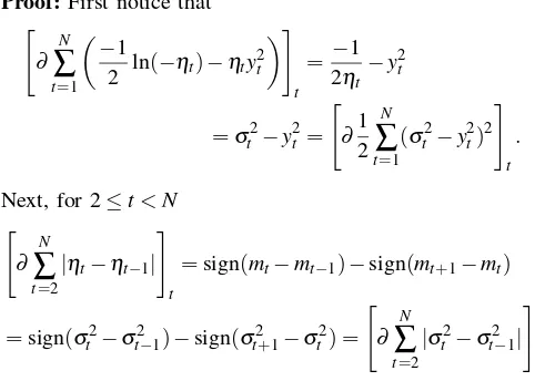
Proof: First notice that "
Here we have used that the sign function defined by (14) only depends on the sign of its argument and (14) implies that the sign is not changed by the transformationσ2
t =−1/(2ηt).
Q.E.D.
Since both optimization problems (10) and (12) are con-vex, Theorem 1 implies that we can re-use algorithms and results for the mean estimation problem to the variance estimation problem (12). For example, it directly follows that
[λ2]max= max
and forλ2≥[λ2]max the constant "empirical variance"
solu-tion
are the optimal solutions to (10) and (12), respectively. From a practical point of view one has to be a bit careful when squaring yt since outliers are amplified.
V. EXAMPLE
Consider a signal {yt} which satisfies yt ∼N(0,σt2), where{σ2
t} is a piece-wise constant sequence:
σ2
timate the variances σ2
1, . . . ,σ10002 . To solve problem (12)
we used CVX, a package for specifying and solving
con-vex programs [7]. Figure 1 shows the resulting estimates of {σ2
Number of measurements
Va
lu
e
Fig. 1. Estimated variance (black line), true variance (blue line) and
measurements (red crosses).
VI. TWOEXTENSIONS
A. Simultaneous Mean and Variance Estimation
The general mean and variance optimization problem (1) is convex and it is possible to findλmaxexpressions. A difficulty
is the termµt2/4ηt in (1) that couples the mean and variance optimization. It is also non-trivial to tune this algorithm in the sense that it is difficult to separate a change in mean from a change in variance based on short data records.
B. The Multi-Variate Case
Assume that the processyt∼N (mt,Σt)∈Rn, that is the mean mt ∈Rn and the covariance matrix Σt ∈Rn×n. The canonical parameters are
µt:=Σ−1t mt Ht:= −1
2 Σ
−1
t .
The corresponding l1 regularized maximum log-likelihood
estimation problem is
minimize
with a large number of unknowns, n+ (n+1)n/2 per n dimension sampleyt.
A problem when trying to generalize the results on the equivalence of variance estimation and mean estimation of
ytyTt is that the ordering relation
Ht+1−Ht= 1 2Σ
−1
t [Σt+1−Σt]Σ−1t+1
does not holds componentwise. Still, the convex problem
minimize
Σ1>0,...,Σn>0
N
∑
i=1
kytyTt −ΣtkF+λ2
N
∑
i=2
kΣt+1−ΣtkF
makes sense as a covariance matrix fitting problem.
VII. CONCLUSIONS
The objective of this contribution has been to introduce the concept of l1 variance filtering and relate this approach
to the problem of l1 mean filtering. The advantage of
the l1 approach is that there are only one or two design
parameters (λ1 and λ2), while classical approaches involve
more user design variables such as thresholds and transition probabilities. The framework presented can also be used for more advanced time-series model estimations such as autoregressive models, see [11]. The number of variables in the multi-variate problem can be huge. Tailored algorithms for this problem based on the alternating direction method of multipliers algorithm, [2], have recently been proposed in [14].
REFERENCES
[1] O. Banerjee, L. El Ghaoui, and A. d’Aspremont. Model selection through sparse maximum likelihood estimation for multivariate
gaus-sian or binary data. Journal of Machine Learning Research, 9:485–
516, 2008.
[2] S. Boyd, N. Parikh, E. Chu, B. Peleato, and J. Eckstein. Distributed op-timization and statistical learning via the alternating direction method
of multipliers.Foundations and Trends in Machine Learning, 3(1):1–
122, 2011.
[3] L. D. Brown.Fundamentals of Statistical Exponential Families, With
Applications in Statistical Decision Theory. Institute of Mathematical Statistics, 1986.
[4] A. P. Dempster. Covariance selection. Biometrics, 28(1):157–175,
1972.
[5] M. Elad. Sparse and Redundant Representations - From Theory to
Applications in Signal and Image Processing. Springer, 2010. [6] J. Friedman, T. Hastie, and R. Tibshirani. Sparse inverse covariance
estimation with the graphical lasso.Biostatistics, 9(3):432–441, 2008.
[7] M. C. Grant and S. P. Boyd. Graph implementations for nonsmooth convex programs. In V. D. Blondel, S. P. Boyd, and H. Kimura, editors,
Recent Advances in Learning and Control (tribute to M. Vidyasagar), pages 95–110. Springer-Verlag, 2008.
[8] F. Gustafsson.Adaptive Filtering and Change Detection. Wiley, 2001.
[9] T. Hastie, R. Tibshirani, and J. H. Friedman. The Elements of
Statistical Learning. Springer, July 2003.
[10] S.-J. Kim, K. Koh, S. Boyd, and D. Gorinevsky. l1 trend filtering.
SIAM Review, 51(2):339–360, 2009.
[11] H. Ohlsson, L. Ljung, and S. Boyd. Segmentation of ARX-models
using sum-of-norms regularization.Automatica, 46:1107 – 1111, April
2010.
[12] P. Stoica and R. Moses. Spectral Analysis of Signals. Prentice Hall,
Upper Saddle River, New Jersey, 2005.
[13] R. Tibshirani, M. Saunders, S. Rosset, J. Zhu, and K. Knight. Sparsity
and smoothness via the fused lasso. Journal of the Royal Statistical
Society: Series B (Statistical Methodology), 67 (Part 1):91–108, 2005.
[14] B. Wahlberg, S. Boyd, M Annergren, and W. Yang. An ADMM
algoritm for a class of total variation regularized estimation problems.