940
EFFECT OF PENALTY FUNCTION PARAMETER IN OBJECTIVE FUNCTION OF SYSTEM IDENTIFICATION
M.F. Abd Samad1, H. Jamaluddin2, R. Ahmad2, M.S. Yaacob2 and A.K.M. Azad3 1
Department of Structure and Materials, Faculty of Mechanical Engineering Universiti Teknikal Malaysia Melaka, Hang Tuah Jaya
76100 Durian Tunggal, Malacca, Malaysia Phone: +(60)6 2346708, Fax: +(60)6 2346884
E-mail: [email protected]
2
Faculty of Mechanical Engineering, Universiti Teknologi Malaysia 81310 UTM Skudai, Johore, Malaysia
Phone: +(60)7 5537782, Fax: +(60)7 5537800
3
College of Engineering and Engineering Technology Northern Illinois University, Illinois 60115, USA
ABSTRACT
The evaluation of an objective function for a particular model allows one to determine the optimality of a model structure with the aim of selecting an adequate model in system identification. Recently, an objective function was introduced that, besides evaluating predictive accuracy, includes a logarithmic penalty function to achieve a suitable balance between the former model’s characteristics and model parsimony. However, the parameter value in the penalty function was made arbitrarily. This paper presents a study on the effect of the penalty function parameter in model structure selection in system identification on a number of simulated models. The search was done using genetic algorithms. A representation of the sensitivity of the penalty function parameter value in model structure selection is given, along with a proposed mathematical function that defines it. A recommendation is made regarding how a suitable penalty function parameter value can be determined.
Keywords: Genetic algorithm; objective function; penalty function; model structure selection; system identification.
INTRODUCTION
System identification is a method of recognising the characteristics of a system, thus producing a quantitative input-output relationship that explains or resembles the
system’s dynamics. The procedure involves the interpretation of observed or measured
941
issue of goodness-of-fit versus model parsimony. This is also referred to as bias (systematic component) versus variance (random component) in an objective function. Many information criterions that are used to evaluate the optimality of a model incorporate such a consideration by including a penalty function, such as the Akaike Information Criterion, Bayesian Information Criterion and Hannan-Quinn Information Criterion (Kapetanios, 2007). As observed in the Bayesian Information Criterion and Hannan-Quinn Information Criterion, an objective function that incorporates a logarithmic penalty function was used in Ahmad et al. (2004b) and Jamaluddin et al. (2007) to cater for the balance between predictive accuracy and model parsimony. However, the parameter values in the penalty function were set arbitrarily. The outcome was a promising balance between the two mentioned characteristics. This outcome is seen to have a potential for further improvement. Different penalty values impose different selective pressures in the population of solutions in constraint-abidance (Li and Gen, 1996). A suitable value of penalty function parameter is thus needed. In this paper, the effectiveness of the objective function is investigated by testing various penalty function parameter values on five simulated dynamic models in the form of a difference equations model. These models are linear and nonlinear autoregressive models with exogenous input (ARX and NARX) (Ljung, 1999). The benefit of using simulated models is the presence of an opportunity to compare the final model directly with the true model. The model structure selection stage requires a robust method that is able to search, within its search space, the model structure that exhibits both predictive accuracy and parsimony with a lower computation burden. This is found in evolutionary computation, which is comprised of genetic algorithm, evolution strategies, evolutionary programming and genetic programming (Sarker et al., 2002). The parameters are estimated using the least squares method.
This paper presents a method that identifies a suitable objective function, specifically the penalty function parameter value. The rest of the paper is organised as follows: Section 2 explains the objective function for model structure selection; Section 3 explains the difference equation model, which is the mathematical model considered here; Section 4 presents the genetic algorithm, which is the search method used in selecting the models based on the specified objective function; Section 5 explains the simulation of system identification; Section 6 provides the results and analysis; and lastly, Section 7 concludes the paper along with a proposed strategy for how to implement the findings in a practical situation and plans or recommendations for future work.
OBJECTIVE FUNCTION
A simple OF in model structure selection is a function that emphasises the accuracy of the prediction of the model. Using the least squares estimation method, the OFis as follows:
OF 2( ) ( ( ) ˆ( ))2
N N
t k t k
ε t y t y t
(1)942
selected model structure, which in turn depends on the variables selected by the search method.
To cater for the balance between predictive accuracy and model parsimony, common objective functions are defined based on bias and variance contributions such as (Ljung, 1999):
( ) P( ) B( )
J D J D J D (2)
where D is the design variable of a certain structure, JP is the variance contribution, and
increases as the number of estimated terms (L), hence the parameters, increases. JB is the
bias contribution and the value decreases as L increases.
In accordance with Equation (1), Jamaluddin et al. (2007) and Ahmad et al. (2004b) define an objective function that evaluates the bias contribution by the sum of squared residuals while the variance contribution is calculated by a penalty function. This is written as follows:
2ˆ
OF PF
N
i i
i
y t y t
(3a)where PF is the penalty function defined as follows:
PFln( )n (3b)
and
n = number of terms satisfying (| aj | < penalty) + 1 (3c)
where | aj | represents the absolute value of the parameter for term j and penalty is a
fixed value termed penalty function parameter. The penalty function penalises terms with the absolute values of the estimated parameter less than the penalty. This is applied so that models that are more parsimonious may be selected over the those that are more accurate but contain many terms.
In Jamaluddin et al. (2007), a trial-and-error approach was adopted in the selection of the penalty function parameter value based on the knowledge that as the value increases, model structures with fewer terms have lower OF. This is true as model structures with more terms, given that ill-conditioning does not occur, have lower residual values but many parameters that are small and considered insignificant to the
model’s predictive accuracy, as based on the parameter in Equation (3c).
NARX MODEL
943
Nonlinear models give much richer possibilities in describing systems and have better flexibility when inferring from a finite data set. The nonlinear version of the ARX model is the NARX (Nonlinear ARX) model. When a time delay exists, it is written as:
( ) *[ ( 1), ( 2),... ( ), ( ),..., ( 1), ( )] allowing d = 1, the nonlinear function for a single-input-single-output NARX model can be expanded into its deterministic form as follows:
input, u, and output, y, sequences (Veres, 1991). The aim in model structure selection is mainly to determine the significant terms to be included in a system’s model.
Before the parameters of the model can be estimated using the least-squares method, the model has to be transformed into a linear regression model as follows:
( )y t T( )t e t( ), ny t N (7)
of noise or disturbance, L is the number of terms, which also determines the size of the parameter vector, and N is the number of data. From here onward, the terms of a model structure may be referred to as regressors.
944
The number of regressors in a NARX model (L) is calculated as follows:
L = M + 1 (8a)
where
1 l
i i
M n
where l = degree of non-linearity (8b)and
ni ni 1(ny nu i 1) i
where no = 1 (8c)
with ny and nu as in Equation (4).
Suppose a NARX system is known to have a non-linearity of 2, maximum order of lag for input, nu = 2, maximum order of lag for output, ny= 2 and time delay, d = 0,
the number of regressors in the model is found to be 15, along with the inclusion of a constant term. Since decisions on the terms are either inclusion or omission, simple binomial theorems apply. Therefore, in a model consisting of L possible terms, the search space is 2L–1, which means there are 32 767 models to choose from.
GENETIC ALGORITHM AND ITS REPRESENTATION OF MODEL STRUCTURE
A genetic algorithm (GA) is a class of artificial intelligence methods that is grouped under a cluster named evolutionary computation. It has the potential to search for the solution to a problem within a small number of trials instead of an enumerative approach. The main characteristics of GA are that it uses binary bit string problem representation, fitness proportional selection in which solutions are assigned a fitness value before further trials are made, and manipulating these selected solutions using a genetic operator called a crossover (Eshelman, 2000; Holland, 1992). In GA, crossover is a process of bits exchange between two strings, and the most common type is one-point crossover where only one and same side of the strings are exchanged. Another important, but considered less provocative, genetic operator is mutation. Mutation refers to the change of bits in a string to another value. GA begins its search of the optimum solution by initialising a set of coded strings where the number of strings is known as the population size, typically denoted popsize. Each string, also called chromosomes, consists of genes that carry an allele or partial information of a potential solution. These chromosomes are evaluated, selected and manipulated until a prespecified number of cycles or generations, typically denoted maxgen. Details of the procedure can be referred to in Goldberg (1989) and Michalewicz (1996).
945
2
1 2 3 4 5 6
7 8 9
2 2
10 11 12 13
14 15
( ) ( 1) ( 2) ( 1) ( 2) ( 1)
( 1) ( 2) ( 1) ( 1) ( 1) ( 2)
( 2) ( 2) ( 1) ( 2) ( 2) ( 1)
( 1) ( 2)
y t a a y t a y t a u t a u t a y t
a y t y t a y t u t a y t u t
a y t a y t u t a y t u t a u t
a u t u t a u
2
(t 2) e t( )
(9)
In a binary-represented GA, the variables and terms are represented by the genes of the chromosome as bit 1 for existence and bit 0 for omission (Ahmad et al., 2004a, 2004b, Jamaluddin et al., 2007). Based on the number of variables and terms in Equation (9), a binary chromosome representation of length lchrom = 15 is generated. The first bit represents the first variable or term and so on, such that chromosome [110 100 001 000 100] represents the following model:
2
1 2 4 9 13
( ) ( 1) ( 1) ( 1) ( 2) ( 1)
y t a a y t a u t a y t u t a u t (10)
The model is completed by the estimation of the parameters a1, a2, a4, a9 and a13.
SIMULATION SETUP
A simple GA (SGA) is used in the simulation. The notion ‘simple’ emphasises that only common characteristics such as those described in Holland (1992) and Eshelman (2000) are applied. To be precise, the operators are roulette-wheel selection, one-point crossover and bit-flipping mutation. The mating preference is based on first-come-first-serve rule (i.e. pairs of chromosomes that are selected first are mated with each other). This mating preference is the mating type of a panmictic population (Bäck and Fogel, 2000). No elitism is used in the algorithm. The fitness of an individual i, denoted fi, is
calculated by subtracting the OF value of the individual from the maximum OF in the population. In mathematical form this is written as follows:
1
i i i
i .. popsize
f max OF OF
(11)
With this setting, individuals with a low OF value have a high fitness.
The probabilities for crossover and mutation used are pc = 0.6 and pm = 0.01. The value for crossover probability is taken from De Jong’s genetic algorithm (De Jong, 1975), claimed as the optimum for both online and offline applications and also recognised as the benchmark for parameter control study using meta-level GA (Grefenstette, 1986). The value for mutation probability is also claimed to be suitable for both online and offline applications in the meta-level GA study. Based on the number of maximum permissible regressors, a population size of 200 and maximum generation of 100 are considered adequate for each penalty.
946
Number of correct regressors: 4 out of a maximum 20 Search space: 1 048 575
Number of correct regressors: 4 out of a maximum 20 Search space: 1 048 575
Number of correct regressors: 5 out of a maximum 21 Search space: 2 097 151
Model 4:
Number of correct regressors: 8 out of a maximum 28 Search space: more than 2×10⁸
Number of correct regressors: 5 out of a maximum 17 Search space: 131 071
The simulation is performed to identify the effect of different values of penalty on the outcome of model structure selection. The identification is made by setting the values of penalty to 0.0001, 0.001, 0.01, 0.1 and 1, consecutively.
947
The following performance indicators are recorded:
(1) Objective function (OF) value of the best selected solution, i.e. the chromosome with the lowest OF value in the final generation;
(2) Error index (EI) of the best selected solution
The error index refers to the square root of the sum of the squared error divided by the sum of the actual output squared. The calculation of EI is as follows:
) (
)) (
ˆ
) ( (
EI 2
2
t y
t y t y
(12)
where y(t) is the actual output value at time t and yˆ is the k-step-ahead predicted output at time t obtained from the least-squares estimation. The value k depends on the specification of a minimum lag of output identified from the model structure selection. This indicator determines the level of accuracy of the final solution. This is also related to a widely-used statistical parameter called the multiple correlation coefficient squared, 2
y
R according to the following function (Ljung, 1999):
Ry2 1EI2
(13)
As such, its relation to OF is:
) ln( ) ( EI
OF 2
y2 t n (14)(3) Numbers of selected regressors in the best chromosome in each generation.
RESULTS AND DISCUSSION
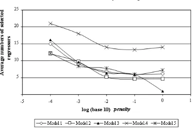
Figure 1 shows the average numbers of selected regressors of the best chromosome in the last 50 generations for different values of log10 penalty. As seen, the numbers of
selected regressors reflect the numbers of correct regressors in the models, respectively. An attempt is hereby made to quantify the relationship between the number of selected regressors and penalty in a mathematical function. In order to do this, several conditions must be fulfilled:
(1) As the value of penalty increases, the function cannot rise upward as this is against the trend in Figure 1.
(2) At any value of penalty, the function cannot intersect the x-axis (axis representing penalty). Its intersection indicates that a negative number of selected regressors can be chosen with a certain value of penalty, which is unacceptable. It can, however, asymptotically converge to any value higher than 0.
948
maximum value of penalty, there is no boundary for the minimum value
of penalty. This indicates that it also converges to a value equal to or
lower than the maximum number of possible regressors.
Figure 1. Average numbers of selected regressors versus log10 penalty.
Given these conditions, an arctangent function is proposed, as follows:
r q penalty
p
( tan (log ))
regressor
selected of
Number 1 10
(15)
while q is the value at which the change of slope is maximum, p and r are determined and constrained by the conditions explained earlier, written as:
maximum number of regressor r 0 (16a)
π
r
p maximum number of regressor- (16b)
p
penalty d
d
)
log (
regressor) selected
of no. (
10
(16c)
Figure 2 shows samples of the fitting of the arctangent function versus log10 penalty for
all simulated models.
For the purpose of further analysis, some inferences are listed here:
949
Model 1 Model 2
Model 3 Model 4
Model 5
Figure 2. Estimated arctangent function fitting of number of selected regressor versus log10 penalty.
(2) With an increase in penalty parameter value, the number of regressors identified as insignificant increases. The number of insignificant regressors in the final model is calculated based on Equation (3). Referring back to Equation (14) which is derived by combining Equations (3a) and (12), rearranging it gives:
950
Replacing n with number of insignificant regressors + 1 (from Equation 3c) and converting to the antilog gives the number of insignificant regressors as follows:
1 regressors
ant insignific of
Number OF EI ()
2 2
y t
e (17b)
(4) A switchover point regarding the number of insignificant regressors and
significant regressors exists such that, at this point, the following function is obtained:
regressors t
significan of
number
regressors ant
insignific of
Number
(18)
where
Number of significant regressors =
number of regressors - number of insignificant regressors (19)
With small penalty parameter values, the number of significant regressors is always higher until a certain penalty parameter value, hereby denoted switchover
penalty, is reached. Beyond this point, the number of insignificant regressors rises.
Within a certain range of this point, the number of true regressors, i.e. correct regressors in the simulated model, with parameters bigger than or equal to the penalty parameter value reaches an agreement with the identified number of significant regressors.
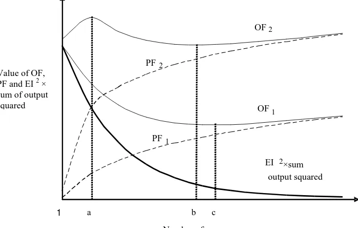
Figure 3. Graph of a general case of the effect of penalty parameter on objective function versus number of regressors.
Number of regressors Value of OF,
PF and EI 2 × sum of output squared
OF2
1
PF 1 PF2
a b
EI
×sum
output squared2 OF1
951
Based on the first two inferences, a graph of a general case of the effect of penalty parameter on model structure selection can be visualised as Figure 3. Both PF1
and PF2 (Equation 3b) refer to the penalty function for given penalty parameter values,
penalty1 and penalty2, respectively, such that penalty2 > penalty1. Since penalty2 is
bigger, PF2 is expected to penalise more regressors, and as other models of more
regressors are evaluated, the penalty grows at a greater pace than PF1. Both OF1 and
OF2 are the objective function values given the penalty parameter values, penalty1 and
penalty2, respectively. For EI2
y2(t) the curve generally converges slowly to 0 asthe number of regressors increases [19]. It shows that the minimum of the curve OF1 is
at c, while OF2 is at b when the number of regressors > a and 1 when the number of
regressors < a. Considering the number of regressors > a, to obtain a parsimonious model (model with b number of regressors), a larger penalty parameter value is required. Note also that the error of prediction represented by EI2
y2(t) in the graph is higher for a parsimonious model. It shows that a compromise in accuracy occurs as parsimony is undertaken.However, at a certain value of penalty parameter, the curve gives two minimum points such as shown with the curve OF2. This is the situation where chromosomes have
the same OFbut different EI. Higher than this penalty parameter value, the minimum is when the number of regressors = 1. It is a scenario when chromosomes with only 1 bit will be selected. It is very likely that this was encountered with Model 3 at penalty = 1. Unlike other models, the number of regressors is too small and too far when compared
to penalty = 0.1 and even far less than the correct number of regressors. The value of the
penalty parameter at which the phenomenon mentioned occurs is hereby called
parsimony penalty. The value is crucial since, with respect to the definition of the
objective function, it determines the most parsimonious model with adequate accuracy. A higher penalty will give a model structure with only 1 variable.
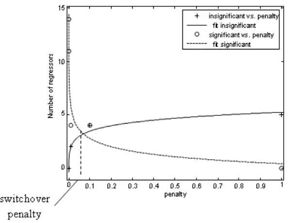
Based on the third inference, a superimposition of the number of insignificant regressors and significant regressors is carried out and fitted to suitable function lines. Due to the boundary of the minimum and maximum number of regressors for each model, an arctangent function is also more appropriate. However, a power function gives an acceptable fit. It is used instead since the purpose is only to find the value of intersection and it gives a better fit to most of these and other preliminary data than any other functions, including linear, exponential and logarithmic. A common form of the power function is used, written as follows:
Number of regressors d (penalty)f g (20)
where d, f and g are model-dependent variables while f is negative for significant regressors and positive for insignificant regressors. The variables are searched by trial-and-error until the best fit is found.
A sample plot of the superimposition using the data from Model 1 is shown in Figure 4. Table 1 gives the values of the switchover penalty where the intersection occurs for each model. A note is made here that caution s required when searching for
switchover penalty for systems that have a low signal-to-noise ratio. Some earlier tests
952
Figure 4. Number of regressors (insignificant and significant) fitted using power functions versus penalty value for Model 1.
Table 1. Switchover penalty for each model.
Models Maximum absolute
parameter value
Minimum absolute
parameter value Switchover penalty
Model 1 0.5 0.3 0.07
Model 2 0.5 0.005 0.09
Model 3 0.07 0.002 0.3
Model 4 0.8 0.2 0.1
Model 5 5 0.0005 0.07
Using this information together with Figure 2, it can be seen that the switchover
penalty can be related to the value q as follows:
10q
switchover penalty > (21)
where q is the value of log10 penalty at which the slope reaches its maximum. It is likely
that since the curve in Figure 4 becomes flatter towards a higher log10 penalty, and by
considering that at a certain penalty value the phenomenon of an OF curve with two minimum points occur, the following becomes true:
Parsimony penalty = Switchover penalty (22)
953
CONCLUSIONS
This paper focuses on an investigation into the effect of the penalty parameter in objective functions towards establishing a suitable objective function in model structure selection. The genetic algorithm has been explained, as the search and optimisation method used in the investigation. The setting of the study has been laid out followed by a discussion of the results. Based on the results, a general case for the effect of the penalty parameter value on the objective function and number of selected regressors has been presented. It shows that when a higher penalty value is applied, a more parsimonious model is selected until a value that gives the most parsimonious and adequate model structure, denoted parsimony penalty. The penalty function parameter is shown to be related to the number of selected regressors by an arctangent function. The study also identifies a penalty value where the number of insignificant regressors is equal to the number of significant regressors, denoted switchover penalty. It was found that the switchover penalty is equivalent to the parsimony penalty, and it can hereby be concluded that by testing SGA on a few initial estimates of penalty value and rerunning it using estimated switchover penalty values, a constant switchover penalty value can be reached. This value represents the suitable penalty value in finding the most parsimonious and adequate model structure. In cases where the smallest tolerable absolute parameter value is known or can be roughly estimated, the penalty parameter value should be set equal to or slightly lower than the parameter value. Future work is aimed at validating the findings on real case studies.
ACKNOWLEDGEMENT
The authors would like to acknowledge the support of the Universiti Teknikal Malaysia Melaka and Universiti Teknologi Malaysia throughout this research, and especially for the UTeM-SLAB sponsorship.
REFERENCES
Ahmad, R., Jamaluddin H. and Hussain, M.A. 2004a. Model structure selection for a discrete-time non-linear system using a genetic algorithm. Proceedings of the Institution of Mechanical Engineers– Part I: Journal of System and Control Engineering, 218(2): 85-98.
Ahmad, R., Jamaluddin H. and Hussain, M.A. 2004b. Selection of a model structure in system identification using memetic algorithm. Proceedings of 2nd International Conference on Artificial Intelligence in Engineering and Technology, Aug 3-5, Universiti Malaysia Sabah, Kota Kinabalu, Sabah, Malaysia, pp. 714-720.
Bäck, T. and Fogel, D.B. 2000. Bäck, T. Fogel D.B. and Michalewicz, Z. (Eds.) Evolutionary computation 1: basic algorithms and operators, Bristol: Institute of Physics.
De Jong, K.A. 1975. An analysis of the behavior of a class of genetic adaptive systems. PhD Thesis. University of Michigan, USA.
Eshelman, L.J. 2000. Genetic Algorithms. Bäck, D.B. Fogel and Z. Michalewicz (Eds.) Evolutionary computation 1: basic algorithms and operators. Bristol: Institute of Physics.
954
Grefenstette, J.J. 1986. Optimization of control parameters for genetic algorithms. IEEE Transactions on Systems, Man and Cybernetics, 16(1): 122-128.
Holland, J.H. 1992. Adaptation in natural and artificial systems. Massachusetts: Institute of Technology, MIT Press, USA.
Hong, X., Mitchell, R.J., Chen, S., Harris, C.J., Li, K. and Irwin, G.W. 2008. Model selection approaches for non-linear system identification: A review. International Journal of Systems Science,39(10): 925-946.
Jamaluddin, H., Abd. Samad, M.F., Ahmad, R. and Yaacob, M.S. 2007. Optimum grouping in a modified genetic algorithm for discrete-time, non-linear system identification. Proceedings of the Institution of Mechanical Engineers– Part I: Journal of System and Control Engineering, 221(7): 975-989.
Johansson, R. 1993. System modeling & identification. New Jersey: Prentice-Hall. Junquera, J.P., Riaño, P.G., Vázquez, E.G. and Escolano, A.Y. 2001. A penalization
criterion based on noise behaviour for model selection. Lecture Notes in Computer Science, 2085: 152-159.
Kapetanios, G. 2007. Variable selection in regression models using nonstandard optimisation of information criteria. Computational Statistics and Data Analysis, 52: 4-15.
Li, Y.X. and Gen, M. 1996. Nonlinear mixed integer programming problem using genetic algorithm and penalty function. IEEE International Conference on Systems, Man and Cybernetics, 4, Oct 14-17, Beijing, China, pp. 2677-2682. Ljung, L. 1999. System identification: theory for the user. 2nd ed. New Jersey: Prentice
Hall.
Michalewicz, Z. 1996. Genetic Algorithms + Data Structures = Evolution Programs, 3rd revised and extended ed. Berlin: Springer-Verlag.
Sarker, R., Mohammadian, M. and Yao X. (Eds.) 2002. Evolutionary optimization, Boston: Kluwer Academic.
Spanos, A. 2010. Akaike-type criteria and the reliability of inference: model selection versus statistical model specification. Journal of Econometrics, 158: 204-220. Veres, S.M. 1991. Structure selection of stochastic dynamic systems: The information