DOI: 10.12928/TELKOMNIKA.v14i1.1731 211
Robust Localization Algorithm Based on Best Length
Optimization for Wireless Sensor Networks
Hua Wu1, Guangyuan Zhang1, Yang Liu*1,2, Xiaoming Wu1, Bo Zhang1,3
1
School of Information Science & Electrical Engineering/Shandong Jiaotong University, Jinan 250357, Shandong, China
2
National Key Laboratory of CNS/ATM/Beihang University
3Schoole of Information Science & Engineering/Shandong University
*e-mail: [email protected]
Abstract
In this paper, a robust range-free localization algorithm by realizing best hop length optimization is proposed for node localization problem in wireless sensor networks (WSNs). This algorithm is derived from classic DV-Hop method but the critical hop length between any relay nodes is accurately computed and refined in space WSNs with arbitrary network connectivity. In case of network parameters hop length between nodes can be derived without complicated computation and further optimized using Kalman filtering in which guarantees robustness even in complicated environment with random node communication range. Especially sensor fusion techniques used has well gained robustness, accuracy, scalability, and power efficiency even without accurate distance or angle measurement which is more suitable in nonlinear conditions and power limited WSNs environment. Simulation results indicate it gained high accuracy compared with DV-Hop and Centroid methods in random communication range conditions which proves it gives characteristic of high robustness. Also it needs relatively little computation time which possesses high efficiency. It can well solve localization problem with many unknown nosed in the network and results prove the theoretical analysis.
Keywords: WSNs, Localization Algorithm, Robustness, Hop Length Optimization
Copyright © 2016 Universitas Ahmad Dahlan. All rights reserved.
1. Introduction
Wireless sensor networks (WSNs) are composed of thousands of tiny and intelligent sensors which are responsible for their organization, configuration and working in order to provide sensing tasks assigned to them. As the development of low-cost and low power sensors, micro-processor and radio frequency circuitry for information transmission, there is a rapid development of WSNs [1], which can be deployed in large numbers and provide unprecedented opportunities for various kind of applications, such as military surveillance, environmental monitoring, habitat monitoring, and structural monitoring etc., [2-5]. There are many challenges in these broad applications.
However sensor node localization has become the most important one, namely how to localize unknown sensors with smallest number of anchors that reduces computation time, communication overheads, and energy consumption but with high localization accuracy has become a hot research topic.
One common way in the world is Global Positioning System (GPS) system. But it is not suitable in WSNs because its performance degrades drastically when receiver is in indoor or located in forest environments. Meanwhile as a result of constraints in size and power consumption, it is unfeasible to equip traditional GPS receivers for all nodes in WSNs. Only those that have the features of well flexibility, convenient maintenance and low-cost update are highly needed. Node localization is one of the important supporting technologies in WSNs.
technology has the characteristics of low cost, no extra hardware requirements, easy to implement, which has been widely applied. In recent years, the sparse transformation and compressed sensing on WSNs locating research have become the academic hotspot.
The other main category is described as range-free. This one only employs distance vector exchange and network connectivity to find the distances between the non-anchor nodes and the anchor nodes to realize node localization by performing a tri-lateration or multi-lateration technique [12, 13] including DV-hop [14], DV-distance, APIT, Euclidean, Amorphous [15], Centroid and others. The differences between based and free are that range-based approaches have higher accuracy but more expensive hardware and higher power consumption are needed and range-free ones need no more complicated hardware and power consumption but with relatively low position estimation error. The parameter that determines its accuracy is derivation of hop length between two nodes.
In this paper, a robust range-free localization algorithm by realizing best hop length optimization, which is high efficient and accurate, is proposed. This algorithm is derived from classic two-dimensional DV-Hop method but the critical hop length between any relay nodes is accurately computed and refined in space WSNs with all sensors deployed randomly and arbitrary network connectivity. In case of network parameters hop length between nodes can be derived without complicated computation and further optimized using Kalman filtering in which guarantees robustness even in complicated environment with random node communication range. Especially sensor fusion techniques used in this paper has well gained robustness, accuracy, scalability, and power efficiency even without accurate distance or angle information which is more suitable in nonlinear conditions.
The contribution of this paper is as follows. A robust 3D node localization based on probability density function analysis is proposed and in this algorithm the best hop length is computed by using regional direction estimation and refined by data fusion technology with relatively low computation time and power consumption. It has a high robust localization accuracy and robustness. The communication range is not fixed but randomly changed, which makes it more suitable in complicted environmets. This break through the biggest restraint in wireless sensor networks.
The rest of the paper is organized as follows. Section II gives some basic problem statement and parameter definitions. Hop length optimization with Kalman filtering are described in Section III. Section IV describes the whole localization algorithm and Section V illustrates the theoretical and simulation results. Finally, conclusions are listed in section VI.
2. Problem Statement and Parameter Definitions 2.1. Problem Statement
In range-free localization algorithms distance between unknown nodes and anchors is the key parameters and becomes the core procedure in the localization algorithms. Normally this distance is computed by hop length and hop counts between unknown and anchors. Once the three similar distances are obtained the unknown coordinates can be computed by multi-lateration methods.
In densely deployed WSNs, a shortest multi-hop path between any pair of the sensor nodes may be existed. By discharging one hop away from the start node, the accumulative distance is likely to be increased by one transmission range [16]. As supposed in the front all nodes have the same property, the distance between any pair of the sensors (StartEnd) can be approximately estimated by the transmission range multiply the corresponding hop counts between them [17]. That is also the core concept of classic DV-Hop propagation algorithm.
But in some bad environment, the density of nodes is very low which is not adequate to construct a straight and shortest multi-hop path between two sensors. In this situation it is impossible for an intermediate sensor to be located close to the boundary of the last one, which makes the estimated distance is far from the true value. It means a lot of localization errors are introduced.
2.2. Parameter Definitions
In the real WSNs, sensor nodes are sprinkled by low flying airplanes or unmanned ground vehicles, all of them are out of control, which makes regularity and topology of the network or the affirmatory pattern hard to be gotten. There are two kinds of nodes in them, one is called anchor node with definitely known position coordinates and the other is unknown nodes which needs to be realized. They are sprinkled together at the same time. Furthermore, all sensor nodes are assumed to be omni-directional, homogeneous and stationary to some extent, which is to say the whole network can be seen as static or regarded as a special snapshot of a mobile ad hoc sensor network. Some parameters used in this algorithm are defined as follows.
1 2 ( , , , N)
N n n n : Total number of sensors in 3D WSNs withnias theithnode.
V L L L: Localization space is a cube as the volume is Vwith side lengthL. /
N V
: Node density in the localization space which subjects to 3D Poisson distribution [18] results from random deployment of sensor nodes in 3D space.
0( )i
V n : The occupied space region with ni node as the center and communication
range ri as its radius which is a random variable up to itself. We can find 3 0( )i 4 i / 3
V n r . In this way the space region of each node is a sphere and any node in it will be seen as its neighbor.
( )
N C : The number of all sensors in one sphere and obviously 3
( ) 4 i / 3
N C r and niis the center of the sphere.
c
N : The number of one sensor’s neighbors and it can be easily computed as
( ) 1
c
N N C .
( , , )
i i i i
A X Y Z : Anchor node Aiwith (X Y Zi, ,i i) as its coordinate. Its coordinates are predefined or from GPS because anchors are a kind of node different from ordinary ones with high power and energy.
In the proposed algorithm the number of hop length needed dealt by Kalman filter for each time is set as 500 to realize optimization. In the model only number of anchor nodes can be changed manually, namely percentage of anchors. The total number of sensors is fixed at 200, which can well represent the real application environment. Note that percentage of anchors in the network is much smaller than that of unknown sensor nodes in the real WSN environment.
3. Hop Length Analysis and Optimization with Kalman Filtering 3.1. Best Hop Length Analysis
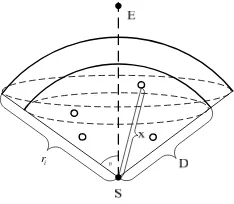
Suppose there is a sensor node indicated as Si with random communication range ri. In this way all nodes in the sphere formed by node Si as its center and random radius riare the neighbors of nodeSi, which is shown in Figure 1. So as shown in Figure 1 once starting node Si is given the hop length towards end node Ei is at each hop is denoted as Riwhich is also a random variable.
i
S
i
r
i
E
i
r
Figure 1. Formation of hop length Figure 2. Best hop length computation
As analyzed before the adjacent hop may not on the straight line connected from node
i
Sto Ei. A neighbor sensor node njwho located nearest its boundary should be selected as the
next hop node. Just as shown in Figure 1 Riis the projection of rion line SE. In Figure 1 it is obvious that R3 R1R2 R ii( 1, 2, 3). However this special sensor node n3should be
neglected for its opposite direction with SE, which means for any relay sensor node, only those neighbors whose position is closer to the ending node E than the current sensor are
considered for the next hop node. Another problem is how to choose between n1and n2. As shown in Fig.1 both n1and n2are in the same space circular cone ASB. Here we call spherical space Sas V1 and compute R1and R2as R1 r1cos1and R2 r2cos2. Finally we select node
2
n as the next hop node for R1R2. That is because it is more close to communication range of node Si.
As analyzed before, parameter is critical because it can decide the size of space region where the best relay hop nodes locate. In order to obtain the rational , we suppose there is a sensor node '
S on the intersection point of SEand sphere S . In this way the next optimum hop length to node Ecan reach its maximum value ri. The special intersection space
region V2, which is formed by sphere S and '
S , can be a perfect estimation of the space step region for source node S. But V1is better than V2to be seen as the optimum space because maximum projection of sensor nodes in (V2V1)on SDis ri/ 2which has low accuracy, which
makes / 3. In this way optimum space hop length can be formed.
3.2. Overview of Kalman Filtering Algorithm
Although WSNs technologies developed very quickly, challenges associated with the scarcity of bandwidth and power in wireless communications have to be addressed. For the state-estimation problems discussed here, observations about a common state are the best hop length computed before. To perform state estimation, sensors may share these observations with each other or to form a fusion center for centralized processing. In either scenario, the communication cost in terms of bandwidth and power required to convey observations is large enough to merit attention. Also in some actual testing environment (temperature, pressure field, magnetic field, etc.), the state changes of sensor node are almost consecutive, which forms a smooth and continuous curve surface. The parameters in Kalman filtering can be performed easily.
The Kalman filtering (KF) offers an elegant, efficient and optimal solution to localization problems in WSNs when the system at hands is distributed and random measurements errors exist [19]. In the paper, the Kalman filter (KF) based approach was selected in order to reduce the effects of hop length errors between anchors and unknown nodes and to obtain property of robustness against existing errors in distance measurements. To explore this point, consider a vector state x n( )Rp at time n and let the kth sensor collect observationsy nk( )Rq. The basic linear state and observation models are:
( ) ( ) ( 1) ( )
Where the driving noise vector u( )n is normal Gaussian noise and uncorrelated across time with covariance matrix Cu( )n while the normal observation noise vk( )n has covariance matrix
( )
v n
C and is uncorrelated across time and sensors. With K vector observations yk( )n
4. The Whole Algorithm Realization
In this part whole algorithm which realize localization for each unknown sensor node is depicted. The best hop length computation is given first and then the whole localization algorithm is described.
4.1. Best Hop Length Computation
As indicated before, all sensors are deployed in 3D WSNs, subjecting to Poisson distribution with node density N V/ [18]. Then, the probability of m sensors located within a sensor ni’s space region, namely 3
Just as the model explained another equation can be written as 3
1 2 i 1 cos / 3
V r .
Similarly, the probability of m sensors can be located in a sphere space section between
( , )of a sensor’s transmission range will be as follows:
Expand it to 3D space as shown in Figure 2. We suppose variable xto be the distance between Siand its next potential forwarding sensor. It is obvious xis a random variable and the probability of x being less than D can be given as Dcan be obtained using following equation.
And the probability density function (PDF) can be computed by differential using the following equation.
As the definition of hop length Ri, the projection on the line connecting the source and the destination nodes, we can easily get Rxcos. Further the best hop length O R( )can be
Finally once node density is given, we can obtain the best hop length using equation (6) for each unknown nodes.
4.2. Realization of the Proposed Algorithm
The proposed localization algorithm with best hop length optimization and Kalman filtering mechanism is described explicitly in this part and some basic symbols are listed first.
i
U : ID of arbitrary unknown node
i
A: ID of arbitrary anchor node
_ _ i
_ _ i
Set Nei U : Set of sensor Ui ’s neighbors
c
H : Hop counts to arbitrary anchor node
L
H : Hop length to arbitrary anchor node
First each unknown sensor node Ui initializes itself by setting its own Num Nei U_ _ i 0
andSet_Nei U_ i {0}. And then they monitor information packages from any anchor nodes to construct the connectivity of the network. Equation (6) is used for each unknown to compute best hop length. Then each anchor node Ai floods information packet over the whole network, which includes ID of anchor nodeAi, hop counts Hc to corresponding anchor node Aiand hop length HL to corresponding anchor nodeAi. As indicated Num Nei U_ _ i 0and
_ _ i {0}
Set Nei U . Once unknown node receives any anchor’s packets it checks if it is from a new anchor. If so, records the ID and renews Hc and HL by using Hc Hc1 and
( )
L L
H H O R . Otherwise HcHc1and Hc are compared. If the former is smaller, renew
c
H or discard the packet. After all of above is finished, unknown node rebroadcasts the packet. The whole process ends when anchor node receives packet from all other anchors. For each time 500 computed best hop length to anchor nodes for each node are stored and dealt using Kalman filter model to perfect the collected distance data to anchor nodes. The most accurate distance estimation can be derived by refining those distance estimations. Finally all the coordinates of all unknown nodes can be derived by other mechanisms, such as tri-angle method and multi-lateration algorithm.
5. Simulation Validation
The simulation is made in the MATLAB (R2008a) software and some assumptions we made are listed first in the following.
a) The whole sensor network is made up of total 200 nodes and the 3D sensing area is 3
100 100 100 m .
b) The percentage of anchors can be changed manually and communication range is a random variable.
c) The observation frequency of Kalman filtering is set as 500.
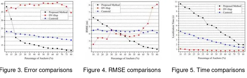
The performance indexes are localization error, root mean square error (RMSE) and the localization time compared with classic DV-Hop and Centroid methods.
Figure 3. Error comparisons Figure 4. RMSE comparisons Figure 5. Time comparisons
Hop. Its localization error changes between 17.5m and 22.5m, which is much better than DV-Hop.
However when percentage of anchors is lower than 10%, the error of our proposed method is the largest. That is because too few anchors cannot help unknown nodes to compute best hop length and introduces lots of accumulated errors. But as the number of anchors increase, its accuracy is getting higher and higher. Just when the value is 20% it becomes the best of the three and it is stable compared with the others. And its error goes on being smaller and smaller. The smallest error of the proposed one is less than 10m, which is only 5% of the side length. The best value of the proposed method is 69.7% and 34.8% better compared with DV-Hop and Centroid.
Figure 4 gives the root mean square error (RMSE) comparisons of the three. DV-Hop presents an upward trend and Centroid keeps stable. The RMSE of Centroid keeps around 4.5m and there are almost no big fluctuations as percentage of anchors changes. DV-Hop fluctuate fiercely and the largest value can reach 8m, which means the environment makes big effects on DV-Hop and sometimes cannot localize itself. Our proposed is definitely the best. It gives a downward trend and better localization performance. The best is less than 2m.
Figure 4 and Figure 5 both depicts accuracy problems of the three. In all proposed method outperforms both the other two. It not only has the least localization error but also has the best RMSE. There is another important index need to be analyzed, namely efficiency. Here we compute the localization time that the three needed, as shown in Figure 5.
It is easy to understand when fewer nodes need to be localized less time will be needed. As shown in Figure 5 the three all give downward trend as unknown nodes get smaller. DV-Hop and Centroid are so simple that they need no complicated computation which makes them need less localization time. DV-Hop needs least time no matter how many nodes need to be localized. It is decided by the algorithm itself. There is no much computation and just one computation process which save a lot of time. Centroid is worse than DV-Hop, because it has to compute the center of some anchors many times. So it consumes more time than DV-Hop. These two algorithms are both fast localization algorithms for their simplicities. And they need less time than most of other proposed algorithms now.
But to some extent our proposed one is the most complex of the three so it needs more computation time with highest accuracy. It not only has localization process but also there is a hop length optimization step and filtering process, which is unavoidable for time consumption. But compared with the other two the time cost is in an accepted range. The worst is about 10.5 seconds which is not a large value. But it realize 90% of all sensor’ localization demand and accuracy is much better than the other two. So it is valuable to obtain much higher accuracy but give up some time performances in the actual use, which is very meaningful.
6. Conclusion
Precise locating target is a precondition for the practice of wireless sensor network, which is connected to the quality of network data collection, data query, data storage, and other applications. The range-free hop length optimization localization algorithm for 3D-WSNs localize the sensors with the help of anchors. In this paper we propose a robust range-free localization algorithm by realizing best hop length optimization, which is high efficient and accuracy. This algorithm is derived from classic two-dimensional DV-Hop method but the critical hop length between any relay nodes is accurately computed and refined with all sensors deployed randomly and arbitrary network connectivity. In case of network parameters hop length between nodes can be derived without complicated computation and further optimized using Kalman filtering in which guarantees robustness even in complicated environment with random node communication range. The results of the simulation experiment indicate that the algorithm proposed in the paper is better than the traditional method in terms of the localization error and energy efficiency.
Acknowledgements
Shandong Province (2014GGX101015) and Natural Science Foundation of Shandong Province (ZR2014FL006).
References
[1] JY Zheng, YE Huang, Y Sun, et al. Error analysis of range-based localisation algorithms in wireless sensor networks. Int. J. Sens. Netw. 2012; 12(2): 78-88.
[2] Stankovic JA. When sensor and actuator networks cover the world. ETRI Journal. 2008; 30: 627-633. [3] I Amundson, J Sallai, X Koutsoukos, A Ledeczi. Mobile sensor waypoint navigation via RF-based
angle ofarrival localization. Int. J. Distrib. Sens. Netw. 2012; (2012): 1-15.
[4] L Cheng, CD Wu, YZ Zhang, Y Wang. Indoor robot localization based on wireless sensor networks. IEEE Trans. Consum. Electron. 57. 2011: 1099-1104.
[5] V Windha Mahyastuty, A Adya Pramudita. Low Energy Adaptive Clustering Hierarchy Routing Protocol for Wireless Sensor Network. TELKOMNIKA. 2014; 12(4): 963-968.
[6] A Bari, S Wazed, A Jaekel, S Bandyopadhyay. A genetic algorithm based approach for energy efficient routing in two-tiered sensor networks. Ad Hoc Networks. 2011; 7(4): 665-676.
[7] Khalid Haseeb, Kamalrulnizam Abu Bakar, Abdul Hanan Abdullah, Adnan Ahmed. Grid Based Cluster Head Selection Mechanism for Wireless Sensor Network. TELKOMNIKA. 2015; 13(1): 269-276.
[8] L Liu. Adaptive Source Location Estimation Based on Compressed Sensing in Wireless Sensor Networks. International Journal of Distributed Sensor Networks. 2012; 31: 123-128.
[9] W Chui, B Chen, C Yang. Robust relative location estimation in wireless sensor networks with inexact position problems. IEEE Transactions on Mobile Computing. 2012; 11(6): 935-946.
[10] S Sarangi, S Kar. Mobility aware routing with partial route preservation in wireless sensor networks. Ubiquitous Computing and Communication Journal. 2011; 6(2): 848-856.
[11] D Ampeliotis, K Berberidis. Low complexity multiple acoustic source localization in sensor networks based on energy measurements. Signal Processing. 2010; 90(4): 1300-1312.
[12] Kashif Naseer Qureshi, Abdul Hanan Abdullah, Raja Waseem Anwar. Wireless Sensor Based Hybrid Architecture for Vehicular Ad hoc Networks. TELKOMNIKA. 2014; 12(4): 942-949.
[13] Sheu JP, Chen PC, Hsu CS. A distributed localization scheme for wireless sensor networks with improved grid-scan and vector-based refinement. IEEE Transactions on Mobile Computing. 2008; 7: 1110-1123.
[14] D Niculescu, B Nath. Ad-hoc positioning system. In Proceeding of IEEE Global Communications Conference (GLOBECOM). 2001: 2926-2931.
[15] Ou CH, Ssu KF. Sensor position determination with flying anchors in three-dimensional wireless sensor networks. IEEE Transactions on Mobile Computing. 2008; 7: 1084-1097.
[16] Yun Wang, Xiaodong Wang, Demin Wang, Dharma P Agrawal. Range-Free Localization Using Expected Hop Progress in Wireless Sensor Networks. IEEE Transactions on Parallel and Distributed Systems. 2009; 20(10).
[17] R Nagpal. Organizing a Global Coordinate System from Local Information on an Amorphous Computer. A.I. Memo1666, MIT A.I. Laboratory. 1999.
[18] Y Wang, X Wang, B Xie, D Wang, DP Agrawal. Intrusion Detection in Homogenous and Heterogeneous Wireless Sensor Networks. IEEE Trans. Mobile Computing. 2008; 7(6).