Measurements of hydrocarbon fluxes by a gradient method
above a northern boreal forest
Janne Rinne
a,∗, Juha-Pekka Tuovinen
a, Tuomas Laurila
a,
Hannele Hakola
a, Mika Aurela
a, Harri Hypén
b,1aAir Quality Research, Finnish Meteorological Institute, Sahaajankatu 20 E, 00810 Helsinki, Finland bFaculty of Forestry, University of Joensuu, P.O. Box 111, 80101 Joensuu, Finland
Received 16 June 1999; received in revised form 10 December 1999; accepted 17 December 1999
Abstract
The boreal vegetation is considered as being a major source of hydrocarbons in the atmosphere. Measurements of vertical fluxes of isoprene and monoterpenes above a northern boreal forest are reported in this paper. Measurements were conducted in northern Finland (67◦58′N, 24◦14′E) near the northern timber lines for conifers. The hydrocarbon fluxes were measured by
the gradient technique. The total daytime fluxes of following four monoterpenes:a- andb-pinene, carene and camphene, were typically 30–60 ng m−2s−1. These compounds represented 60–80% of the total monoterpenes in the ambient air. The estimated
uncertainty of isoprene fluxes exceeded observed fluxes several times, the mean daytime flux being 4±20 ng m−2s−1. The
error sources of the measured hydrocarbon fluxes are discussed. The most important source of uncertainty was the hydrocarbon sampling and analysis due to low concentration gradients. © 2000 Published by Elsevier Science B.V. All rights reserved.
Keywords:Biogenic VOCs; Flux measurements; Boreal forests; Biogenic emissions; Uncertainty analysis
1. Introduction
Boreal vegetation is assessed as being a major source of volatile organic compounds (VOCs) in the atmosphere (Guenther et al., 1995) and in some countries its contribution to the total national VOC emissions is very significant (Lindfors et al., 1995; Simpson et al., 1995). For instance, almost the whole of Finland belongs to the boreal vegetation zone
∗Corresponding author. Present address: Atmospheric Chemistry Division, National Center for Atmospheric Research, 1850 Table Mesa Dr., Boulder CO 80303, USA. Tel.:+1-303-497-1413; fax: +1-303-497-1477.
E-mail address:[email protected] (J. Rinne)
1Finnish Forest Association, Salomonkatu 17 B, 00100 Helsinki, Finland.
and 66% of the land area of 305 000 km2is covered by forests. Simpson et al. (1995) estimated that in Finland biogenic VOC emissions are twice as high as anthropogenic emissions. Over the whole globe there is a total of ca. 15.8×10⁶km2 of boreal forest (Archibold, 1995).
The biogenic VOCs can have a strong effect on the atmospheric chemistry, for example on the production of tropospheric ozone (Chameides et al., 1992). They can also be a major source of organic aerosols and their oxidation affects hydroxyl radical concentrations in the troposphere (Fehsenfeld et al., 1992).
Much work has been carried out using the cuvette technique to obtain the emission rates for different plant and VOC species (e.g., Isidorov et al., 1985; Juuti et al., 1990; Guenther et al., 1991; Janson, 1993; Street
et al., 1996; Hakola et al., 1998). Isoprene emissions are generally considered to be temperature and light dependent, whereas monoterpene emissions are often taken to be dependent on temperature only (Guenther et al., 1991). Using species-specific emission factors, it is possible to calculate the VOC emissions for a specific site or a larger area using forest information and weather data.
Measurements of the vertical fluxes of VOCs above the forest canopy are needed to verify the emissions calculated using species-specific emission factors and forest inventory data. Published results on these ver-tical fluxes are still rather sparse although there has been recent progress (e.g., Fuentes et al., 1996; Gold-stein et al., 1996; Guenther et al., 1996; Reichmann et al., 1996; Cao et al., 1997; Ciccioli et al., 1997; Schween et al., 1997; Valentini et al., 1997; Guenther and Hills, 1998; Rinne et al., 1999).
In this work we present the ambient air concentra-tions of isoprene and monoterpenes and their vertical fluxes as measured by a gradient method in the north-ern boreal zone in Finland 150 km north of the Arctic Circle. As an integral part of the study, the basic micrometeorological assumptions are tested and a systematic approach has been taken to identify and quantify the potential error sources.
2. The experiment
2.1. The site
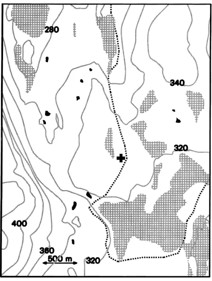
The flux measurements were conducted dur-ing the period of the 9–20 July 1996 near the Pallas-Ounastunturi National Park in northern Finland (Finnish Lapland). The measurement site (67◦58′N, 24◦14′E, 330 m above sea level (asl)), hereafter re-ferred to as Kenttärova, was situated on a low ridge between two hills, 350 and 440 m high (Fig. 1). The area is 150 km north of the Arctic Circle and close to the northern timber lines of Norway spruce (Picea abies) and Scots pine (Pinus sylvestris). The forest around the measurement site was composed mainly of mountain birch (Betula pubenscens subsp. czere-panovii), which is a subspecies of downy birch (B. pubenscens), Siberian spruce (P. abies subsp. obo-vata), which is a subspecies of Norway spruce, and Scots pine. The average tree density, leaf dry biomass,
Fig. 1. Map of the micrometeorological measurement site, Kent-tärova. The black cross indicates the location of the measurement masts. The checked areas are wetlands, black areas indicate ponds and the broken line is a small road. Numbers on the height con-tours are metres above sea level.
etc., are shown in Table 1. The average height of the canopy at the measurement site was estimated to be 13 m.
Near to the measurement site is situated the Pallas-Sodankylä GAW (Global Atmosphere Watch) station, where ambient air VOC concentrations are sampled twice a week on an open mountain top at 560 m asl, about 200–300 m above the surrounding terrain (Laurila et al., 1995). The light hydrocarbons (up to C5) are analyzed from whole air samples col-lected into evacuated electropolished stainless steel canisters using gas chromatography with flame ioniza-tion detector (GC/FID). The heavier hydrocarbons are collected onto Tenax adsorbent and analyzed by gas chromatography with mass spectrometer (GC/MS).
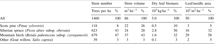
Table 1
Forest inventory data from the micrometeorological measurement sitea
Stem number Stem volume Dry leaf biomass Leaf/needle area Trees per ha % m3ha−1 % 103kg ha−1 % 103m2ha−1 %
All 1460 100 86 100 5.0 100 50 100
Scots pine (Pinus sylvestris) 118 8 22 26 0.5 10 3 5
Siberian spruce (Picea abiessubsp.obovata) 623 43 24 28 2.8 56 16 32 Mountain birch (Betula pubenscenssubsp.czerepanovii) 679 47 37 43 1.6 32 29 58
Other (Goat willow,Salix caprea) 39 3 3 3 0.1 3 2 5
aThe leaf areas are two-sided and needle areas based on the shape of needles.
measurement site in 1961–1990 was 18.5◦C (Finnish Meteorological Institute, 1991). The average yearly rainfall was 450 mm, of which a large part fell as snow. The average rainfall in July was 72 mm.
2.2. Methods
2.2.1. Theory
We applied the gradient method, in which vertical fluxes are inferred from the vertical gradient of the mean concentration
Fc= −Kc∂c¯
∂z, (1)
wherec¯is the mean concentration of the trace gas,Fc
is its vertical flux, upward flux being positive, andKc
is the turbulent exchange coefficient.
There are two common ways of obtaining the turbu-lent exchange coefficient in the surface layer. The most direct way is the modified Bowen-ratio method (e.g., Goldstein et al., 1995) which however requires accu-rate measurements of gradients of another gas (e.g., H2O, CO2), and when these gradients are small a large error can be introduced into the exchange coefficients. The other method of obtaining the turbulent ex-change coefficient is to use the universal flux–gradient relationships. In this way it is possible to determine the turbulent exchange coefficients without requiring gradient measurements, if the momentum and sensi-ble heat fluxes are measured directly. The vertical flux of a trace gasFccan be written as (e.g., Fuentes et al., 1996),
Fc= −ku∗(c(z¯ 2)− ¯c(z1))
ln((z2−d)/(z1−d))
+ψh((z1−d)/L)−ψh((z2−d)/L)
, (2)
wherek is the von Kármán constant, u∗ is the fric-tion velocity, c(z¯ 1) and c(z¯ 2) are the hydrocarbon concentrations measured at heights z1 and z2, d is the zero-plane displacement height,ψhis the integral form of Monin–Obukhov stability function for heat, which is assumed to be the same for trace gases, andL
is the Obukhov length.ψhis calculated using integral forms of the Businger–Dyer equations (e.g., Garratt, 1994) and the fluxes of heat (buoyancy) and momen-tum measured by the eddy covariance technique. An important prerequisite of these approaches is that the vertical fluxes remain constant within the observation layer.
Near very rough surfaces, such as forest canopies, the flux gradient laws tend to break down (Garratt, 1980; Chen and Schwerdtfeger, 1989; Högström et al., 1989; Cellier and Brunet, 1992; Mölder et al., 1998; Simpson et al., 1998). The layer in which these laws are not directly applicable is called the roughness sub-layer (RSL). The flux obtained by Eq. (1) can be cor-rected by multiplying by an enhancement factor
γ =8s
8, (3)
where8sis the dimensionless gradient of a scalar ac-cording to the Monin–Obukhov similarity theory and
8is that according to the measurements. The observed
γ-coefficients vary from unity to 3 depending on the measurement height and type of the forest (Simpson et al., 1998, and references therein).
the correction function for heat and water vapour to have form
γ = z∗−d
z−d . (4)
This equation is also supported by the study by Mölder et al. (1998). Garratt (1980) suggested earlier an Eq. (5)
Using these equations it is possible to calculate the mean enhancement factor, Ŵ, by integrating the
γ-coefficient between the measurement heights z1 andz2. Forz1<z∗<z2we have enhancement factor is used to correct fluxes calculated using Eq. (2).
2.2.2. Hydrocarbon sampling
The measurement system consisted of two masts 18 and 31 m high, situated 2 m apart. The vertical gradients of the hydrocarbon concentrations were estimated using samples taken at these two heights. Light hydrocarbons were sampled in 0.85 l stainless steel canisters via teflon tubing from both heights. The canisters were pressurized to about 200 kPa and the flow was controlled by a needle valve. This sim-ple method was calibrated using a pressure sensor and it was found to keep the flow into the canis-ter reasonably constant. The sampling time for light hydrocarbons was 25 min. Terpenes were sampled into 250 mg of Tenax TA using automated samplers (Perkin Elmer STS 25) and pumps with an automatic flow control system (Ametek Alpha-2) situated at both measurement heights. The sampling time was 30 min. At the near-by Pallas-Sodankylä GAW station VOCs are sampled twice a week using similar methods. The chemical analysis of the samples was conducted by GC/FID (canisters) and GC/MS (Tenax) as described by Hakola et al. (1998).
2.2.3. Micrometeorological measurements
To determine the turbulent exchange coefficients, the vertical fluxes of momentum and buoyancy
were measured by the eddy covariance method us-ing three-dimensional acoustic anemometers-thermo-meters (ATI SWS-211) at both measurement heights (18 and 31 m). The vertical fluxes of H2O, CO2 and O3were also measured by eddy covariance technique. For H2O and CO2 a sensor based on the differential absorption of IR-radiation (Li-Cor LI-6262) was used, while the O3 fluctuations were determined using a sensor based on chemiluminescence (GFAS OS-G-2) at 31 m. Details of the measurement system and data processing procedures are presented by Aurela et al. (1996, 1998) and Tuovinen et al. (1998). The averag-ing time for the flux measurements was 30 min.
Other meteorological parameters, such as the temperature and humidity inside the forest (Vaisala HMP35D), the ground temperature (Campbell 107), the ground water status (Watermark gypsum block) and photosynthetically active radiation (Li-Cor LI-190SZ), were also measured.
The displacement height was assumed to be two-third of the canopy height, i.e. 8.7 m (e.g., Garratt, 1994).
3. Results
3.1. Meteorological measurements
3.1.1. Conditions during the campaign
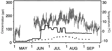
Temperatures during the measurement period were relatively low (Fig. 2) due to the northerly winds, which prevailed during the campaign. The observed cloudiness at Muonio weather station varied from half
cloudy to cloudy and there was some rain on several days. The only days during the campaign with no rain were 16, 19, and 20 July. The available soil moisture was sufficient to prevent plants from suffering water stress.
The PAR and fluxes measured by the eddy covari-ance method showed a clear diurnal cycle in spite of the long daylight period (Fig. 3), as did the air temperature. The carbon dioxide flux was typically
−0.2 mg m−2s−1 in the afternoon and slightly posi-tive (i.e. upwards) at night. The typical evaporation rate in the afternoon was 0.14 mm h−1. The daily cy-cle of the ozone flux was not as systematic as that of the H2O flux, the hourly median values in the daytime ranging from−0.2 to−0.4mg m−2s−1. The values of these fluxes were of the same order as those measured by Aurela et al. (1996) above a Scots pine stand in eastern Finland.
Fig. 3. Hourly medians (solid lines) and upper and lower quartiles (dashed lines) of photosynthetically active radiation (PAR) and fluxes measured by the eddy covariance method (H: sensible heat flux,u∗: friction velocity) 11–19 July 1996. The positive sign on eddy covariance fluxes means upward flux.
3.1.2. Validity of the micrometeorological assumptions
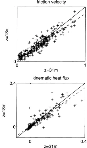
As mentioned earlier, an important prerequisite of the gradient method is that the vertical fluxes remain constant within the observation layer. To validate the constant-flux assumption we compared the friction ve-locities, heat fluxes and roughness lengths measured at both measurement heights.
The measured sensible heat fluxes were similar at both measurement heights, as were the momentum fluxes. Only a small bias was found (Fig. 4). The mean ratio of friction velocity measured at the upper height to that at the lower,ru∗ = u∗31 m/u∗18 m, was 1.05, and the same ratio for the sensible heat flux,rH =
w′T′31 m/w′T′18 m, was 1.03.
Table 2
The ratios of momentum and sensible heat fluxes measured at 31 m to those measured at 18 m (ru∗ =u∗31 m/u∗18 m andrH= w′T′
31 m/w′T′18 m) and roughness heights (z0) measured at both measurement heightsa
Wind direction Stability
z<−0.02 −0.02<z<0.02 z>0.02 ru∗ rH ru∗ z0(18 m) z0(31 m) ru∗ rH
315–45◦ 1.06 1.20 1.11 1.3 m 1.3 m 0.94 1.00 (51) (39) (23) (23) (23) (56) (5) 45–200◦ 1.08 1.30 1.10 1.3 m 1.0 m 1.24 –
(53) (46) (12) (12) (12) (15) (0) 200–315◦ 1.10 1.15 1.27 1.7 m 1.9 m 0.85 0.78
(44) (35) (4) (4) (4) (19) (8) aNumber of observations are in parenthesis.
homogeneous for a little over 1 km, and even beyond that the ground was still reasonably flat. In the second sector (45–200◦), the forest changed after 800 m into an area of open wetlands, while in the third sector (200–315◦) the steep slope of Mustakero hill rose at a distance of 1 km. Using the the footprint formulae by Schuepp et al. (1990) for neutral conditions, 75% of the flux measured at 31 m originated within 1 km of the masts. For the 18 m height, 75% of the measured flux originated within 300 m of the masts. For unstable conditions these source area radii are even shorter.
From Table 2 we notice thatru∗is close to unity in unstable conditions. In near-neutral and stable condi-tions there are larger deviacondi-tions, but for northerly wind directions the ratio is still reasonably close to unity. The ratio of friction velocities is usually closer to unity than the ratio of heat fluxes, which may be due to the large scatter of the heat fluxes also seen in Fig. 4.
As the second test, the roughness length was cal-culated from eddy covariance measurements at both heights. The roughness length was calculated using the equation
z0(z)=(z−d)exp
−u(z)k u∗(z)
−ψm[ζ (z)]
, (7)
whereζ =(z−d)/L, and accepting near-neutral ob-servations only(|ζ|<0.02).
The roughness lengths obtained from the upper and lower level measurements were closest to each other in northerly wind directions, in which z0 = 1.3 m (Table 2). The differences between the roughness
Fig. 4. Comparison between friction velocities and kine-matic heat fluxes (w′T′) measured at two heights. The solid line indicates a 1:1 relation, while the dashed line indi-cates the best fit relations: u∗18 m = 0.85u∗31 m+0.039 m s−1, w′T′18 m=0.88w′T′31 m+0.0043 Km s−1.
lengths derived from different measurement heights in the other two wind direction classes may arise from nonhomogeneity of the surface roughness. Changing the value of the zero plane displacement height within the limits given by Jarvis et al. (1976) did not explain the observed differences. The close fit of the rough-ness lengths measured in northerly wind directions gives also confidence in the choice of the zero-plane displacement height.
To summarize, we conclude that northerly wind di-rections seem to be the most reliable for gradient mea-surements, and the VOC fluxes presented further were measured under those conditions.
had systematic errors and could not be used in this comparison. The height of the RSL was approximated byz∗−d=4δ(Cellier and Brunet, 1992) and the for-est inventory data (Table 1). The dominant trees at the site were Siberian spruces and Scots pines. Their stem number per ha was about 700. This leads to δ≈4 m and therefore toz∗≈24.7 m. Thus the upper measure-ment level seems to be above the RSL according to Cellier and Brunet (1992).
The Ŵ-coefficients calculated using Eqs. (4)–(6) with measurement heights of 18 and 31 m and a RSL height of 24.7 m were 1.21 according to Gar-ratt (1980) and 1.15 according to Cellier and Brunet (1992). Theγ-coefficients obtained by Simpson et al. (1998) ranged between 1.1 and 1.5 for measurement height to canopy height ratios between 1.4 and 2.4.
The turbulent exchange coefficients for heat ob-tained from the theoretical flux–gradient relationships (Eqs. (1) and (2)) were compared with those obtained using temperature gradients and sensible heat fluxes. The data used for comparison is filtered to meet the fol-lowing criteria: Wind direction is 315–45◦;|ζ|>0.2;
u∗>0.1 m s−1and measurement time is 8:00–18:00 or 22:00–4:00 hours. The least-square line for the data showed that theŴ-coefficient for heat was 1.20, which is close to the values obtained earlier. There is, how-ever, a large scatter andr2is only 0.39. The deviation from the universal flux–gradient relationship was not generally dependent on stability, though there was an increase with strongest instability.
As there are both theoretical and practical limita-tions in the direct method of obtaining the turbulent exchange coefficient for heat, the coefficients obtained from the flux–gradient relationships are used for hy-drocarbon flux calculations. These coefficients are cor-rected by multiplying them by an enhancement factor ofŴ=1.2 based on the findings mentioned earlier.
Finally, one should be aware of the fact that chemical reactions of trace gases in the surface layer can also lead to a breakdown of the con-stant trace gas flux layer. In the present case, how-ever, the timescale for vertical mixing, τm, is much shorter than the timescale for chemical degrada-tion. If we take the measurement height zm≈30 m and the friction velocity u∗≈0.1–1.0 m s−1 then the timescale τm=zm/u∗≈30–300 s≈0.5–5 min. Accord-ing to Finlayson-Pitts and Pitts (1986), the typical lifetimes fora- andb-pinene and carene range from
3 to 18 h. The chemical reactions seem therefore to be of minor importance.
3.2. Hydrocarbon concentrations
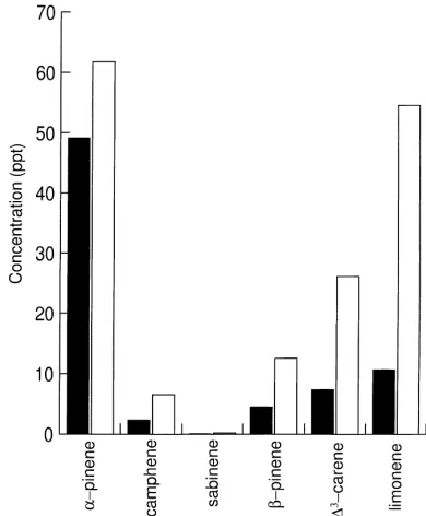
The total ambient air monoterpene concentra-tions measured at the Pallas-Sodankylä GAW sta-tion were higher than the isoprene concentrasta-tions (Fig. 2). This suggests that the total monoterpene emissions are higher than those of isoprene. At the micrometeorological measurement site, Kenttärova, the monoterpene concentrations were slightly higher than at the GAW station and the composition of the total monoterpene concentration differed from that observed on the mountain top (Fig. 5). At the GAW station most of the monoterpenes were in the form of a-pinene. It was also the most common monoterpene at the Kenttärova site, but there other species con-tributed more to the total monoterpene concentration, limonene being almost as abundant asa-pinene. The reason for this behaviour may lie in the differences of reactivities of these monoterpenes. Because the re-activity ofa-pinene in O3and OH reactions is lower
than that of limonene (Atkinson, 1994), a-pinene is more evenly distributed in the atmospheric boundary layer, whereas limonene profiles are affected more by chemistry.
3.3. Hydrocarbon fluxes and their uncertainty
Before the results of the VOC flux measurements are presented, a systematic approach into the poten-tial error sources of these VOC flux measurements is taken. This is accomplished by identifying the error sources and discussing their relative importance.
3.3.1. Sources of uncertainty
For the gradient method, the sources of uncertainty can be divided into those of the gradient itself and those due to the turbulent exchange coefficient. The latter can be further divided into uncertainties originat-ing from the flux measurements and those arisoriginat-ing from the parametrisations. A list of uncertainties relevant for the present data is presented for these categories in Table 3, partly based on the review by Businger (1986) of the errors related to micrometeorological techniques. Unfulfilled micrometeorological assump-tions may be considered as the third source of uncer-tainty. These were addressed in Section 3.1.2 and are also dealt with within the data screening procedures. As it is not possible to assess the possible remaining
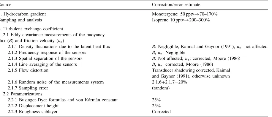
Table 3
Uncertainties of the VOC fluxes measured at Kenttärova
Source Correction/error estimate
1. Hydrocarbon gradient Monoterpene: 50 pptv→70–170%
Sampling and analysis Isoprene 10 pptv→200–300%
2. Turbulent exchange coefficient
2.1 Eddy covariance measurements of the buoyancy flux (B) and friction velocity (u∗)
2.1.1 Density fluctuations due to the latent heat flux B: Negligible, Kaimal and Gaynor (1991);u∗: not affected 2.1.2 Frequency response of the sensors B,u∗: Negligible
2.1.3 Spatial separation of the sensors B: Not affected;u∗: corrected, Moore (1986) 2.1.4 Line averaging of the sensors B,u∗: corrected, Moore (1986)
2.1.5 Flow distortion Transducer shadowing corrected, Kaimal and Gaynor (1991), otherwise unknown 2.1.6 Random noise of the measurements system 2.1.6+2.1.7=20%
2.1.7 Sampling error (random)
2.2 Parametrizations
2.2.1 Businger-Dyer formulas and von K´arm´an constant 25%
2.2.2 Displacement height 25%
2.2.3 Roughness sublayer Corrected
errors in a systematic way, for the following discus-sion we assume no further uncertainty due to non-ideal flow conditions.
For this data set, the most important error source affecting the measured fluxes is the chemical sam-pling and analysis of the hydrocarbons. This is due to the small concentration differences between the mea-surement levels, as compared to the resolution of the chemical analysis. In order to reduce this uncertainty, we calculated the flux as the sum of four monoter-penes (a- andb-pinene, carene and camphene). These compounds make up 60–80% of the total atmospheric monoterpene concentration above the forest and their gradients also correlate with each other. The latter was not true for limonene, which also had problems in the chemical analysis and was therefore not included in the sum.
the accuracy of the monoterpene gradients. For iso-prene, the uncertainty of the analysis was estimated at 10 pptv by analyzing several canisters twice. With the range of gradients observed at Kenttärova, these val-ues lead to uncertainties of 200–300% in the isoprene gradient and 70–170% in the monoterpene gradient.
In the eddy covariance measurements of the mo-mentum and buoyancy (virtual temperature) fluxes for the exchange coefficient, a number of the potential er-rors characteristic of this technique can be identified, many of which can be routinely corrected for. These are listed as Items 2.1.1–2.1.7 in Table 3. A sonic anemometer, such as the type used here, also provides a measurement of the virtual temperature to a close ap-proximation, even without concomitant measurement of humidity fluctuations (Kaimal and Gaynor, 1991). This makes it possible to obtain in a consistent way the fluxes needed for the exchange coefficient.
There is no temporal delay between the anemome-ter signals nor any spatial sensor separation within the heat flux measurement, but the momentum flux is af-fected by the sensor configuration of the SWS-211, in which the vertical and horizontal sonic paths are sep-arated. This together with the line averaging over the paths leads to attenuation of high-frequency fluctua-tions and consequently to a small systematic flux loss. We have corrected for this based on the procedure by Moore (1986), as detailed by Tuovinen et al. (1998).
The random noise in the measurement system and sampling errors introduce a random uncertainty into the flux measurements. It has been estimated that the natural run-to-run variability for the 30-min averag-ing period is approximately 10–20% at heights of 5–10 m in ideal daytime conditions, and this can be significantly increased by sensor noise (Wesely and Hart, 1985; Businger, 1986). We assume that the ran-dom variability in the momentum and heat flux data is dominated by sampling effects, and that after the corrections listed in Table 3 this is the main source of uncertainty in the eddy covariance measurements employed in this study. To summarize, we adopt a value of 20% for the further uncertainty analysis.
The use of universal flux–gradient relationships in-troduces an uncertainty that can lead to systematic er-rors in the turbulent exchange coefficient. There exists a consensus on the functional form of these relation-ships, but a range of values have been reported for the related empirical constants (e.g., Businger et al., 1971;
Dyer, 1974; Wieringa, 1980; Högström, 1988; Oncley et al., 1996). This variability is taken here as an in-dication of the uncertainty due to parametrisation. In principle, the constants used in the Businger–Dyer for-mulae, together with the von Kármán constant, should be treated as one parameter set, since in practice they are not determined independently. We assessed that the variability between the parameter sets leads up to 25% differences in the calculated exchange coefficients.
The zero-plane displacement height is here taken as an independent parameter. According to Jarvis et al. (1976) the reported ratio of the displacement height and the mean canopy height ranges from 0.61 to 0.92. For our data, this leads to differences of 25% in the ex-change coefficient. Similar roughness lengths obtained from both measurement heights give confidence in the value of 0.67 adopted here.
Using the standard error propagation method we can now sum up the uncertainties arising from the Items 1, 2.1.6, 2.1.7 and 2.2 in the Table 3. The summing is done separately for each data point.
3.3.2. Observed hydrocarbon fluxes
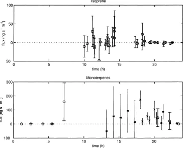
During daytime, values of monoterpene fluxes range from negative to 150 ng m−2s−1 (Fig. 6). At night the fluxes are close to zero. Nightly fluxes should be treated with care because of light winds and stable conditions latter leading to longer footprint areas. Be-cause of the large uncertainties, these values should be taken as order-of-magnitude estimates. The uncer-tainty of isoprene flux was much higher than observed fluxes. The small fluxes observed are at least partly due to the low temperatures (6–16◦C) during the mea-surements. The lower uncertainty of terpene fluxes on 13 July is due to the more cloudy weather and lower mixing in the boundary layer which lead to larger gra-dient relative to emission. During these measurements there was also some light rain.
Fig. 6. Measured fluxes of isoprene (upper panel) and total fluxes of four terpenes (a- andb-pinene, camphene and carene; lower panel; crosses: 13 July, stars: 16 July and circles 17–18 July) with their error estimates.
flux measurements of isoprene was 4±20 ng m−2s−1. The observed terpene fluxes are an order of magni-tude higher than observed isoprene fluxes. This is in line with the ambient air concentrations observed at the Pallas-Sodankylä GAW station.
To study the influence of the individual monoter-pene species on the total flux, the data from 13 July is used due to its relatively low uncertainty. During these measurements a-pinene was the dominant monoter-pene emitted, making 49% of the monotermonoter-pene flux. The abundance of other species were13-carene: 30%; b-pinene: 16%; and camphene: 5%.
The temperature dependence of the monoterpene emission is generally described by the equation
E=E30exp[β(T −30◦C)], (8)
where E is emission rate, E30 is the emission nor-malized to 30◦C,T is the leaf temperature (◦C) and
β is empirically-determined coefficient (Guenther et al., 1991). The temperature dependency in most of the published measurements is of the same order (β≈0.1–0.2) (e.g., Isidorov et al., 1985; Juuti et al., 1990; Guenther et al., 1991; Janson, 1993; Hakola et al., 1998).
Most of the emission factors published are for the total monoterpene emission but some of them are for specific terpenes. It might be better to use emission factors for the total monoterpene emission, as Hakola et al. (1998) have observed large differences between emitted terpene species even within a single plant species (B. pendula), while the total monoterpene emission rate was more conservative.
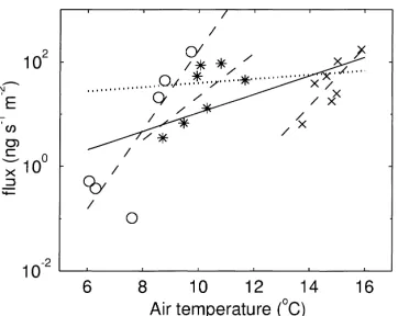
Fig. 7. Temperature dependencies (Eq. (8)) of measured terpene fluxes. The solid line is fitted to the whole data (β=0.41 in Eq. (8)) and the dashed lines to separate runs: 13 July (+) (β=1.3), 16 July (*) (β=0.96) and 17–18 July (o) (β=1.7). The dotted line is based onβ=0.09 andE30=240 ng s−1m−2.
data set is closest to those published. One possible reason for these differences is the use of air tempera-ture instead of leaf temperatempera-ture. Asβ-coefficients for individual runs are systematically higher than those for whole data set, it seems possible that other factors than temperature are needed to explain the emission rates. The mean emission normalized to 30◦C using b=0.09◦C−1, which is commonly used in the emis-sion models, is 240 ng s−1m−2.
4. Conclusions
A measurement campaign has been conducted in the northern boreal zone in order to estimate biogenic VOC emissions by the micrometeorological gradient method. The VOC concentrations were measured at 18 and 31 m using GC-MS with cartridges filled with Tenax TA and stainless steel canisters. The turbu-lent exchange coefficient was calculated using sur-face layer flux–gradient relationships and the fluxes of heat and momentum measured by the eddy covari-ance method. The micrometeorological assumptions were shown to have been satisfactorily fulfilled and the measurement system worked well.
A typical total flux of four important monoterpenes was 30–60 ng m−2s−1 during the daytime and close to zero at night. The low emissions observed were at least partly due to the low temperatures. The most
abundant monoterpene in the emission wasa-pinene,
13-carene being the second. The temperature de-pendency of the measured fluxes was stronger than usually found using cuvette techniques. The mean daytime isoprene flux was very low, 4±20 ng m−2s−1. This is in line with the observed ambient air isoprene concentrations, as they are much lower than the total monoterpene concentrations.
The sources of uncertainty of measured VOC fluxes leading to either random or systematic errors, have been discussed. The most important sources of un-certainty were the hydrocarbon gradients, due to the small concentration gradients. The flux values pre-sented should be taken as order-of-magnitude esti-mates. To reduce the effect of random uncertainties, longer time series would be useful.
Acknowledgements
This work was a part of the BIPHOREP research project funded by the Academy of Finland and the European Commission (contract ENV4-CT95-0022). Janne Rinne thanks Maj and Tor Nessling Foundation for financial support. We also thank Ari Halm, Jukka Kiiski and Anne-Mari Mäkelä of the Finnish Meteo-rological Institute for technical assistance. The staff at the Pallasjärvi Research Station of the Finnish Forest Research Institute have been very helpful.
References
Archibold, O.W., 1995. Ecology of World Vegetation. Chapman & Hall, London, 510 pp.
Atkinson, R., 1994. Gas-Phase Tropospheric Chemistry of Organic Compounds, J. Phys. Chem. Reference Data, Monograph No. 2, 216 pp.
Aurela, M., Laurila, T., Tuovinen, J.-P., 1996. Measurements of O3, CO2 and H2O fluxes over a Scots pine stand in Eastern Finland by the micrometeorological eddy covariance method. Silva Fennica 30, 97–108.
Aurela, M., Tuovinen, J.-P., Laurila, T., 1998. Carbon dioxide exchange in a subarctic peatland ecosystem in Northern Europe measured by the eddy covariance technique. J. Geophys. Res. 103, 11289–11301.
Businger, J.A., 1986. Evaluation of the accuracy with which dry deposition can be measured with current micrometeorological techniques. J. Climate Appl. Meteorol. 25, 1100–1124. Businger, J.A., Wyngaard, J.C., Izumi, Y., Bradley, E.F., 1971.
Cao, X.-L., Boissard, C., Juan, A.J., Hewitt, C.N., Gallagher, M., 1997. Biogenic emissions of volatile organic compounds from gorse (Ulex europaeus): diurnal emission fluxes at Kelling Heath, England. J. Geophys. Res. 102, 18903–18915. Cellier, P., Brunet, Y., 1992. Flux-gradient relationships above tall
plant canopies. Agric. For. Meteorol. 58, 93–117.
Chameides, W.L., Fehsenfeld, F., Rodgers, M., Cardelino, C., Martinez, J., Parrish, D., Lonneman, W., Lawson, D.R., Rasmussen, R.A., Zimmerman, P., Greenberg, J., Middleton, P., Wang, T., 1992. Ozone precursor relationships in the ambient atmosphere. J. Geophys. Res. 97, 6037–6055.
Chen, F., Schwerdtfeger, P., 1989. Flux-gradient relationships for momentum and heat over a rough natural surface. Q. J. R. Meteorol. Soc. 115, 335–352.
Ciccioli, P., Concetta, F., Brancaleoni, E., Cecinato, A., Frattoni, M., Cieslik, S., Kotzias, D., Seufert, G., Foster, P., Steinbrecher, R., 1997. Biogenic emissions from the Mediterranean pseudosteppe ecosystem present in Castelporziano. Atmos. Environ. 31, 167–175.
Dyer, A.J., 1974. A review of flux profile relations. Boundary-Layer Meteorol. 1, 363–372.
Fehsenfeld, F., Calvert, J., Fall, R., Goldan, P., Guenther, A., Hewitt, N., Lamb, B., Liu, S., Trainer, M., Westberg, H., Zimmerman, P., 1992. Emissions of volatile organic compounds from vegetation and the implications for atmospheric chemistry. Global Biogeochem. Cycles 6, 389–430.
Finlayson-Pitts, B.J., Pitts, J.N., 1986. Atmospheric Chemistry: Fundamentals and Experimental Techniques, Wiley/Inter-science, New York, Chichester, Brisbane, Toronto, Singapore, 1098 pp.
Finnish Meteorological Institute, 1991. Climatological Statistics in Finland 1961–1990, Finnish Meteorological Institute, Meteorological Yearbooks, Vol. 90.
Fuentes, J.D., Wang, D., Neumann, H.H., Gillespie, T.J., Den Hartog, G., Dann, T.F., 1996. Ambient biogenic hydrocarbons and isoprene emissions from a mixed deciduous forest. J. Atmos. Chem. 25, 67–95.
Garratt, J.R., 1980. Surface influence upon vertical profiles in the atmospheric near-surface layer. Q. J. R. Meteorol. Soc. 106, 803–819.
Garratt, J.R., 1994. The Atmospheric Boundary Layer, 1st paperback edition with corrections. Cambridge University Press, Cambridge, 316 pp.
Goldstein, A.H., Daube, B.C., Munger, J.W., Wofsy, S.C., 1995. Automated in-situ monitoring of atmospheric non-methane hydrocarbon concentrations and gradients. J. Atmos. Chem. 21, 43–59.
Goldstein, A.H., Fan, S.M., Goulden, M.L., Munger, J.W., Wofsy, S.C., 1996. Emissions of ethene, propene and 1-butene by a midlatitude forest. J. Geophys. Res. 101, 9149–9157. Guenther, A.B., Hills, A.J., 1998. Eddy covariance measurement
of isoprene fluxes. J. Geophys. Res. 103, 13145–13152. Guenther, A.B., Monson, R.K., Fall, R., 1991. Isoprene and
monoterpene emission rate variability: observations with eucalyptus and emission rate algorithm development. J. Geophys. Res. 96, 10799–10808.
Guenther, A., Baugh, W., Davis, K., Hampton, G., Harley, P., Klinger, L., Vierling, L., Zimmerman, P., Allwine, E., Dilts,
S., Lamb, B., Westberg, H., Baldocchi, D., Geron, C., Pierce, T., 1996. Isoprene fluxes measured by enclosure, relaxed eddy accumulation, surface layer gradient, mixed layer gradient, and mixed layer mass balance techniques. J. Geophys. Res. 101, 18555–18567.
Guenther, A., Hewitt, C.N., Erickson, D., Fall, R., Geron, C., Graedel, T., Harley, P., Klinger, L., Lerdau, M., McKay, W.A., Pierce, T., Scholes, B., Steinbrecher, R., Tallamraju, R., Taylor, J., Zimmerman, P., 1995. A global model of natural volatile organic compound emissions. J. Geophys. Res. 100, 8873– 8892.
Hakola, H., Rinne, J., Laurila, T., 1998. The hydrocarbon emission rates of tea-leafed willow (Salix phylicifolia), silver birch (Betula pendula) and European aspen (Populus tremula). Atmos. Environ. 32, 1825–1833.
Högström, U., 1988. Non-dimensional wind and temperature profiles in the atmospheric surface layer: a re-evaluation. Boundary-Layer Meteorol. 42, 55–78.
Högström, U., Bergström, H., Smedman, A.S., Halldin, S., Lindroth, A., 1989. Turbulent exchange above a pine forest I. Fluxes and gradients. Boundary-Layer Meteorol. 49, 197–217. Isidorov, V.A., Zenkevich, I.G., Ioffe, B.V., 1985. Volatile organic compounds in the atmosphere of forest. Atmos. Environ. 19, 1–8.
Janson, R., 1993. Monoterpene emission of Scots pine and Norwegian spruce. J. Geophys. Res. 98, 2839–2850. Jarvis, P.G., James, G.B., Landsberg, J.J., 1976. Coniferous forest.
In: Monteith, J.L. (Ed.), Vegetation and the Atmosphere. Academic Press, New York, pp. 171–240.
Juuti, S., Arey, J., Atkinson, R., 1990. Monoterpene emission rate measurements from a Monterey pine. J. Geophys Res. 95, 7515–7519.
Kaimal, J.C., Gaynor, J.E., 1991. Another look at sonic thermometry. Boundary-Layer Meteorol. 56, 401–410. Laurila, T., Plathan, P., Hakola, H., Koskinen, T., Lättilä, H., 1995.
Pallas, a site for studies of photochemically-active trace species in the European Arctic. EUROTRAC Newsletter, pp. 2–4. Lindfors, V., Laurila, T., Hongisto, M., 1995. Estimation of
hydrocarbon emissions from forests in Finland. In: Tolvanen, M., Anttila, P., Kämäri, P. (Eds.), Proceedings of the 10th World Clean Air Congress, 28 May–2 June 1995. Finnish Air Pollution Prevention Society, Helsinki, Vol. 1.
Mölder, M., Grelle, A., Lindroth, A., Halldin, S., 1998. Flux-profile relationships over a boreal forest — roughness sublayer corrections. Agric. For. Meteorol., submitted, for publication. Moore, C.J., 1986. Frequency response corrections for eddy
correlation systems. Boundary-Layer Meteorol. 37, 17–35. Oncley, S.P., Friehe, C.A., Larue, J.C., Businger, J.A., Istweire,
E.C., Chang, S.S., 1996. Surface-layer fluxes, profiles, and turbulence measurements over uniform terrain under near-neutral conditions. J. Atmos. Sci. 53, 1029–1044. Reichmann, A., Steinbrecher, R., Zelger, M., 1996. Design and
Rinne, J., Hakola, H., Laurila, T., 1999. Vertical fluxes of monoterpenes above a Scots pine stand in the boreal vegetation zone. Phys. Chem. Earth 24, 711–716.
Schuepp, P.H., Leclerc, M.Y., MacPherson, J.I., Desjardins, R.L., 1990. Footprint prediction of scalar fluxes from analytical solutions of the diffusion equation. Boundary Layer-Meteorol. 50, 355–373.
Schween, J.H., Dlugi, R., Hewitt, C.N., Foster, P., 1997. Determination and accuracy of VOC-fluxes above the pine/oak forest at Castelporziano. Atmos. Environ. 31, 199–215. Simpson, D., Guenther, A., Hewitt, C.N., Steinbrecher, R., 1995.
Biogenic emissions in Europe 1. Estimates and uncertainties. J. Geophys. Res. 100, 22875–22890.
Simpson, I.J., Thurtell, G.W., Neumann, H.H., Den Hartog, G., Edwards, G.C., 1998. The validity of similarity theory in the roughness sublayer above forests. Boundary-Layer Meteorol. 87, 69–99.
Street, R.A., Ducham, S.A., Hewitt, C.N., 1996. Laboratory and field studies of volatile organic compound emissions from Sitka
spruce (Picea sitchensis Bong.) in the United Kingdom. J. Geophys. Res. 101, 22799–22806.
Tuovinen, J.-P., Aurela, M., Laurila, T., 1998. Resistances to ozone deposition to a flark fen in the northern aapa mire zone. J. Geophys. Res. 103, 16953–16966.
Valentini, R., Greco, S., Seufert, G., Bertin, N., Ciccioli, P., Cecinato, A., Brancaleoni, E., Frattoni, M., 1997. Fluxes of biogenic VOC from Mediterranean vegetation by trap enrichment relaxed eddy accumulation. Atmos. Environ. 31, 229–238.
Wesely, M.L., Hart, R.L., 1985. Variability of short term eddy-correlation estimates of mass exchange. In: Hutchison, B., Hicks, B. (Eds.), The Forest-Atmosphere Interaction. D. Reidel Publishing Company, Dordrecht, Netherlands, pp. 591–612.