FAST RADIOMETRY GUIDED FUSION OF DISPARITY IMAGES
Stephan Schmida, Dieter Fritschb
a Daimler AG - [email protected] b
Institute for Photogrammetry, University of Stuttgart - [email protected]
Commission III, WG III/1
KEY WORDS:Disparity fusion, multi-view stereo, real-time stereo, machine vision, photo-consistency
ABSTRACT:
Previous work on disparity map fusion has mostly focused on geometric or statistical properties of disparity maps. Since failure of stereo algorithms is often consistent in many frames of a scene, it cannot be detected by such methods. Instead, we propose to use radiometric information from the original camera images together with externally supplied camera pose information to detect mismatches. As radiometric information is local information, the computations in the proposed algorithm for disparity fusion can be decoupled and parallelized to a very large degree, which allows us to easily achieve real-time performance.
1. INTRODUCTION
For several years, it has been possible to obtain high-quality dense distance measurements using stereo algorithms such as semi-global matching (SGM) (Hirschmüller, 2005). However, the resolution of real time implementations is limited by available processing power. What is worse, even top performing algorithms such as SGM suffer from frequent mismatches in certain situations. In stereo computation with moving or multiple cameras, it is com-mon to fuse several disparity / depth images together to improve accuracy and to remove matching artifacts. Artifact removal is particularly important if the result is intended to be viewed by humans, for example in 3D city reconstruction.
Most methods for depth map fusion use geometric or statistical considerations to process the depth images, often without use of the information contained in the original color images. We pro-pose a novel approach which uses color information to identify mismatched pixels, which we denote radiometry guided dispar-ity fusion (RGDF). As color information alone provides a robust way to distinguish foreground from background, RGDF is able to eliminate mismatches even in the presence of moving objects in a scene.
The paper is organized as follows: In the next section, we briefly discuss related work. Section 3 introduces the core RGDF al-gorithm and describes its application to the temporal filtering of disparity images. Section 4 outlines the algorithmic implementa-tion and the setup used for input data generaimplementa-tion. Secimplementa-tion 5 dis-cusses the results of the method using qualitative and quantitative evaluation.
2. RELATED WORK
The problem of fusing several depth / disparity images has been studied extensively in the context of multi-view stereo (MVS). This is due to the fact that MVS methods which optimize photo-consistency for multiple images simultaneously (cf. e.g. (Collins, 1996), (Rumpler et al., 2011), (Toldo et al., 2013)) typically re-quire a large amout of computational effort. Therefore, a popular approach is to first perform stereo matching for certain pairs of in-put images and to fuse the obtained disparity images in a second step. With the advent of high-quality real time stereo algorithms
such as semi-global matching (Hirschmüller, 2005) and inexpen-sive RGB-D cameras such as the Kinect, real time algorithms for disparity fusion have gained interest. In addition to dedicate depth fusion algorithms such as (Merrell et al., 2007, Unger et al., 2010, Tagscherer, 2014), depth image fusion algorithms are often presented in the context of a 3D reconstruction method as a post-processing step for integrating multiple depth images.
In the depth image fusion algorithm (Merrell et al., 2007), can-didates of depth values for a view are evaluated using their oc-clusion of samples from other views. Based on these ococ-clusion relations the plausibility of the candidates is evaluated, with up to one candidate being selected as result. Since its introduction, this method has become very popular and has been used to fuse depth images from a variety of depth image sources.
Among the statistical approaches for merging depth images, there are two main branches. Methods using clustering in image space are popular due to their speed advantages, cf. e.g. (Unger et al., 2010), (Rothermel et al., 2012), (Tagscherer, 2014). Variants that perceive stereo disparity images as noisy approximations of the true disparity image which is assumed to satisfy certain spatial regularity conditions have been applied successfully to e.g. aerial imagery, cf. e.g. (Pock et al., 2011), (Zach et al., 2007). Meth-ods using clustering in object space such as (Hilton et al., 1996), (Rumpler et al., 2013), (Wheeler et al., 1998) handle complex geometry more easily, but at the cost of increased computational complexity.
The 3D reconstruction method (Furukawa and Ponce, 2010) uses a region-growing approach. Before triangulation, erroneous gions are detected by enforcing visibility constraints and by re-jecting solitary patches as outliers.
In the multi-view stereo method presented in (Liu et al., 2009), depth image merging for a view is performed by first rejecting solitary points and points whose normals are slanted more than 45◦
away from the camera. Then, the fused depth value is chosen from the remaining candidates by selecting the one which maxi-mizes photoconsistency.
image. (Schmeing and Jiang, 2013) oversegments the color im-age and averim-ages depth over each segment. (Chen et al., 2015) uses an energy minimization approach. The energy term con-sist of a fidelity term, which models the deviation from the input depth data and incorporates color information, and a regulariza-tion term, which is based on the color image based depth image denoising method proposed in (Liu et al., 2010).
3. METHOD 3.1 Design and basic operation
The design goals of the method presented here are given as fol-lows:
• Strong robustness to erroneous data: This is neccessary in particular to remedy the frequently poor edge quality of stereo algorithms such as SGM and to deal with unmodelled be-haviour such as moving objects.
• Use of ’local’ computations to facilitate scaling and paral-lelization.
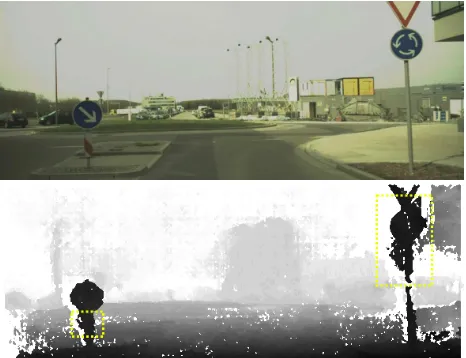
It is a well-known fact that in many scenes, different objects can be distinguished by their color, that is by radiometric informa-tion. Disparity images obtained from stereo algorithms often suffer from systematic errors. For example in traffic scenes, a common situation is that well-textured objects (signs, pedestri-ans, lamp poles) are in front of an untextured or almost untex-tured background (road surface, walls of buildings, sky), cf. fig-ure 1. In these situations, the disparity of the background
pix-Figure 1. Example of SGM failure at object borders in front of a uniform background. Pixel intensities range from near to far from dark to bright. Pixel without disparity value (invalid disparities) are white.
els is ambiguous so SGM cannot detect where the foreground object ends. Thus SGM usually assigns the foreground dispar-ity not only to the pixels of the foreground object, but also to a certain area around the foreground object. In contrast, radiomet-ric information is the result of a direct measurement and is thus essentially error-free. The RGDF algorithm compares radiomet-ric values for samples from different views to distinguish correct disparity matches from incorrect matches. This yields a robust
way of detecting incorrect disparity matches. Furthermore, ra-diometric information is local information, which allows us to parallelize the computations to a very large degree.
RGDF operates on the following data:
• a number of input views (IV), each consisting of a radiomet-ric image, a corresponding disparity1image and the corre-sponding camera pose;
• the reference view (RV), consisting of a radiometric image and the corresponding camera pose.
The output of RGDF is a fused disparity image for the reference view.
In our implementation, the IV disparity images are computed by SGM from the image pair of a stereo camera. We use the left color images as radiometric images and determine the cam-era poses using a GNSS / IMU combination. Our application of RGDF is to filter a temporal sequence of images. The reference view corresponds to the most recent camera image and the input views correspond to older images. Since the essential require-ment though is that the input views provide sufficient coverage of the reference view, we do not require the reference view to con-tain a disparity image. If a disparity image is available for the reference image, this is formulated as an additional input view. Furthermore, note that the resolution of radiometric image and disparity images in both the input views and the reference view may differ.
RGDF transforms the points of the input views to the reference view. There, they are assigned to a pixel of the RV disparity image. The points assigned to a pixel of the RV disparity image are averaged in order to compute its value. Since this averaging is a delicate step, we will discuss it beforehand: We will use variants of the arithmetic mean for averaging (cf. also section 3.4). An arithmetic mean has the form
P
s∈samplesvalue(s)
P
s∈samples1
. (1)
Simlarly, a weighted arithmetic mean has the form
P
s∈samplesweight(s)·value(s)
P
s∈samplesweight(s)
. (2)
Thus, computing such averages can be divided into two steps:
1. Sum certain values over all samples.
2. Compute the final value from the sums.
In the same way, the RGDF algorithm is divided into two steps. In the first step, all points of the input views are processed sepa-rately and the desired sums are computed via accumulation. Then in the second step, the final value is computed for each pixel of the disparity image of the reference view. Since this accumulation is done simultaneously for all pixels of the RV disparity image, we use a buffer which provides a set of accumulation variables for each pixel of the RV disparity image. We call this the accu-mulation buffer.
1
3.2 First step: Processing IVs and accumulation
In the first step, the data of the IVs are processed. We select the pixel centers of the radiometric image as sampling points of an IV, since the resolution of the radiometric image is typically higher than or equal to the resolution of the disparity image. Given such a point of an IV, the following substeps are performed.
i) The disparity value and radiometric values are sampled at the position of the point. If no disparity value is available for the point (invalid disparity), the point is discarded.
ii) The point is transformed to the reference view, that is into a pair of coordinates on the reference image (this is the trans-formed position) together with a transtrans-formed disparity value. Transformation beween 3D Euclidean coordinates and the triple consisting of camera coordinates and disparity may be performed in homogeneous coordinates by multiplication with an augmented versionC˜of the camera matrix resp. its inverse:
Here,fis the focal length,cx,cyare the coordinates of the principal point andbis the stereo baseline. Rigid transfor-mations (rotations, translations and composites of these) in Euclidean space may be performed in homogeneus coordi-nates by multiplication with a block matrix of the form
˜
where the rotation matrixRdescribes the rotation compo-nent and the translation vectorv describes the translation component. Multiplying all these matrices, we may perform the transformation from an IV to the RV in homogeneous coordinates by multiplication with a single4×4-matrix.
iii) Radiometric values are sampled at the position of the trans-formed point on the reference view. These values are com-pared with the IV radiometric value. If the dissimilarity of the values exceeds a given threshold, the point is discarded. In our implementation, we use the following measure of RGB dissimilarity. LetIbe the IV RGB color vector. LetR be the RV RGB color vector. Letαbe the angle betweenI andR. We set
to be the normalized color difference. We set
di:=
R
kRk·
R−I
kRk (6)
to be the normalized intensity difference. Then, we define the RGB dissimilarity to be
d(R, I) :=pd2
c+ (0.2di)2. (7)
Note that the color component receives a larger weight than the intensity component to provide a certain measure of
bright-ness invariance (e.g. due to varying camera exposure times). More sophisticated dissimilarity metrics may be used e.g. if information about sensor characteristics or color distribution in the scene is available. Sinced(R, I)is a scalar value, the dissimilarity threshold is a dimensionless number.
iv) Calculate the values for accumulation. This is the trans-formed disparity value and the value one as weight. I.e. we do not average linear distance values, but disparity values. This is due to the fact that we use disparity values as in-put and the transformation from disparities to linear dispar-ity values has a singulardispar-ity at the dispardispar-ity value zero. This is particularly problematic since precision is lowest for dis-parity values near zero (cf. also (Sibley, 2007, section 2.3)). Averaging the reciprocal of linear distance, that is disparity, avoids this singularity.
Weighted arithmetic means can be computed by using weights
6
= 1and by multiplying the averaged values with the weights before accumulation as discussed in eq. (2). Though we do not use non-unit weights, weighted averaging may be used to e.g. replace or augment the thresholding in substep iii).
v) The point is assigned to the RV disparity image pixel that is nearest to its transformed position. The values generated in step iv) are added to the accumulation variables of the RV disparity image pixel in the accumulation buffer.
Substeps i)-iv) can be performed independently for all points of the IVs. Only in substep v), the points are collected at the pixels of the RV disparity image. This structure facilitates massive par-allelization and is especially suited for GPU hardware, cf. section 4.1.
3.3 Second step: Computing averages from accumulated val-ues
The second step consists of computing the final values of the en-tries of the RV disparity image from the corresponding accumu-lated values in the accumulation buffer as discussed above. Since this is done independently for each pixel of the RV disparity im-age, it can be readily parallelized.
3.4 Methods for averaging
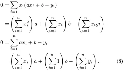
Above, we demonstrated how to efficiently compute arithmetic means by using accumulation. To demonstrate the flexibility of this approach, we discuss how to use it to compute other quan-tities. For example, the König-Huygens formula / Steiner trans-lation theorem may be used to compute variance by accumula-tion. In this way, e.g. the disparity averaging method presented in (Sibley, 2007, section 2.2.3) may be implemented, which uses both arithmetic mean and variance to obtain significantly im-proved convergence rates. Lastly, let us discuss linear regres-sion: Given samples(xi, yi),i∈ {1, . . . , n}, we want to deter-mine the values fora, bwhich minimize the quadratic functional
1 2
Pn
i=1(axi+b−yi) 2
func-tional with respect toaandbyields the equations
This system of linear equations is uniquely solvable if at least two of thexi, i ∈ {1, . . . , n}are distinct. For details, confer e.g. (Kenney and Keeping, 1962). Note that all coefficients can be computed by accumulation, so linear regression may be com-puted using accumulation.
3.5 Variants for filtering
We investigate two variants of filtering of stereo sequences. Each of these use the left camera images as radiometric images and use SGM to generate input disparity images. Each variant gen-erates a disparity image for the most recent (current) left camera image, i.e. the current left image is used as RV radiometic image. The first variant (’basic’) uses as input the lastnframes including the current frame together with the corresponding SGM disparity image as IV images. The difference of the second variant (’feed-back’) from the basic variant is that once a filtered disparity image is computed for the current frame, it is used to replace the SGM image of the current frame in the IVs. Thus for subsequent frames in the stereo sequence, this filtered disparity image is used as part of an input view. The feedback mechanism is interesting since firstly, it uses the ’best’ available disparity images as input. Sec-ondly, the feedback mechanism feeds results as input back into the data used for filtering which might allow erroneous values to remain indefinitely in the pipeline. Additionally, we implemented a third variant (’low latency’) which differs from the basic variant in that no IV is given for the RV. This way, RGDF can be started as soon as the RV radiometric image becomes available without having to wait for completion of the stereo algorithm, which may be used to reduce latency. This variant yields reasonable results, cf. e.g. figure 2, but due to the large amount of invalid dispari-ties, (typically∼20%), it is difficult to evaluate properly, so we concentrate on the first and second variant.
Figure 2. Result of ’low latency’ variant on a frame of sequence 2011_09_26_drive_0013 of the KITTI raw data recordings
4. TEST SETUP AND IMPLEMENTATION 4.1 Implementation of RGDF
Our implementation uses a mixed CPU / GPU implementation. While a suitably optimized pure CPU implementation should reach real-time performance on a modern CPU, we use a GPU imple-mentation for step one of the algorithm since this offers more flexible texture sampling as well as virtually unlimited process-ing power. Step two is implemented on the CPU.
The GPU implementation of step one is written in OpenGL 3.3 and apart from non-essential integer arithmetic, only OpenGL 2.0 functionality is used. We use point sprite rendering to process the points of the IVs. Substeps i)-ii) are performed in the ver-tex processing stage. Substeps iii)-iv) are performed in the pixel processing stage. Substep v) is performed by the alpha blending functionality of the render output units.
We performed some rough performance measurements on a sys-tem featuring an Intel Core i7-4770K @ 3.5 GHz as CPU and a Nvidia GeForce GTX 780 as GPU. Using a image size of 0.47 megapixels for radiometric and disparity images of both IVs and RV, the processing time increases from about 8.5 milliseconds for one input view approximately linearly to about 16 milliseconds for 40 input views. While this is well within real time perfor-mance, it is far below the throughput the GPU should be capable of, which highlights that the implementation is written with the aim of providing algorithmic flexibility instead of ultimate per-formance (in fact, about 70% of CPU time is usually spent in the graphics driver stack).
4.2 Test setup
We generate disparity images from the images of a front-facing vehicle-mounted stereo camera. For quantitative evaluation, we use the raw data recordings of the KITTI Vision Benchmark Suite (Geiger et al., 2013), which feature a pair of color cameras as stereo camera and a GNSS / IMU system for pose determination. For development and real time testing, we use the built-in driver assistance stereo camera of a commercial car and a GNSS / IMU system for pose determination. For stereo matching, we use a variant of the FPGA-based implementation of SGM presented in (Gehrig et al., 2009). Note that it generates disparity images at half the resolution of the camera images. For example for the 1242x375 images of the KITTI dataset, the resolution of the of the IV disparity images is 621x187.
5. EXPERIMENTAL EVALUATION
We evaluate the method qualitatively using visual inspection. Fur-thermore, for quantitative evaluation and discussion of parame-ter choice, we run tests on sequences of the rectified and synced KITTI raw data recordings (Geiger et al., 2013).
Each frame of a sequence of the KITTI raw data recordings pro-vides two pairs of rectified stereo camera images (one grayscale pair and one color pair), a GNSS / IMU provided pose and about 100k points of LIDAR measurements. We use the color image pair as input of SGM to compute disparity images. The disparity images are fused by RGDF using the left color images for radio-metric data and the GNSS / IMU data for camera poses. We use the LIDAR data as ground truth reference. The vertical field of view (FOV) of the LIDAR is about+3◦
to−25◦
, so roughly the lower half of the camera FOV is covered.
Pixels without disparity value (invalid disparities) are treated as outliers. However, the datasets in the KITTI benchmark pro-vide densely interpolated LIDAR data as ground truth whereas the KITTI raw data recordings only provide the (sparse) LIDAR data. So instead of evaluating all pixels of a disparity image as in the KITTI benchmark, we evaluate only the pixels for which a LI-DAR measurement is available. In the image parts covered by the LIDAR FOV (below+3◦
elevation), the LIDAR measurements cover about 7% of the pixels.
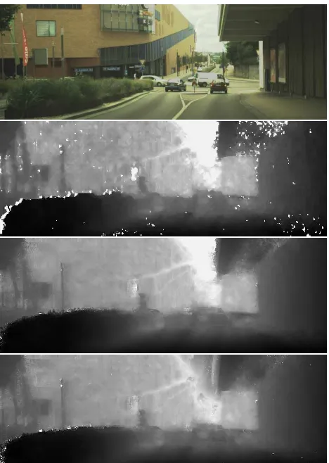
Figure 3. Picture detail of traffic scene. From top to bottom: Left color image, SGM image, output of basic variant (10 IVs, thresh-old=0.1), output of feedback variant (5 IVs, threshold=0.07). Note the contours of the sign on the left hand side
basic variant
color dissimilarity threshold
0.05 0.1 0.15 0.2
#
IVs
5 0.269 0.239 0.235 0.247 10 0.258 0.224 0.227 0.254 15 0.255 0.229 0.245 0.288 20 0.256 0.239 0.267 0.323
feedback variant
color dissimilarity threshold
0.05 0.1 0.15 0.2
#
IVs
5 0.260 0.225 0.243 0.310 10 0.260 0.291 0.430 0.501 15 0.267 0.335 0.466 0.574 20 0.276 0.379 0.509 0.604
Table 4. Outlier ratios of the basic and feedback variant in se-quence 2011_09_26_drive_0013 of the KITTI raw data record-ings for various parameters
Figure 5. Picture detail of traffic scene. See fig. 3 for parameter description. Note the poles and flags on the left hand side.
Table 4 shows an example of the influence of the color dissim-ilarity threshold and of the number of IVs. In this scene, SGM has an outlier ratio of 0.312. The basic variant of RGDF shows best results for the threshold value 0.1 and for 10 IVs. Further-more, deviation from these optimal parameters causes only weak worsening of performance. The best outlier ratio of the feed-back variant is very close to the best outlier ratio of the basic variant. It is reached at as few as 5 IVs and a threshold value of 0.1. However, the feedback variant is much more sensitive to the choice of parameters. Unsuitable choice of parameters cause the feedback variant to diverge (this behaviour shows clearly in frame-by-frame analysis as runaway error growth).
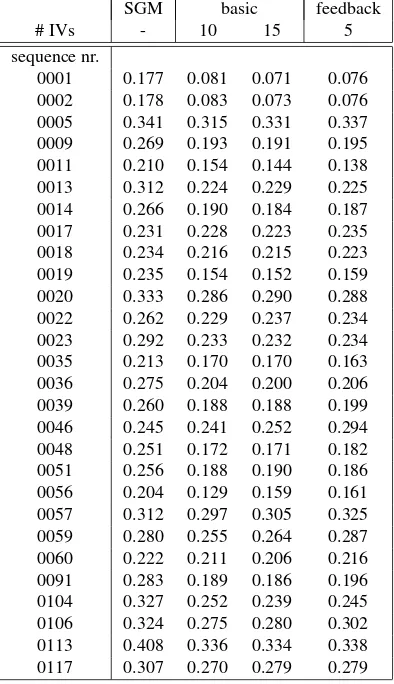
In table 8, we compare selected configurations of the fusion al-gorithm against the half-resolution SGM we use for input data generation. For brevity, we discuss only select representative se-quences. Sequence 0001 is a simple static scene. In sequence 0005, a car and a bicycle is driving in front of the vehicle. In sequence 0013, the vehicle is overtaken by two cars. In sequence 0017, the vehicle is standing still at a road intersection, with cars crossing. Note that the tested RGDF configurations perform simi-lar. Furthermore, even in adverse conditions such as in sequences 0005 and 0017, the outlier ratio does not exceed or only barely ex-ceeds the outlier ratio of the input SGM data. Overall, the ’basic’ variant almost never worsens the outlier ratio, while the ’feed-back’ variant worsens the outlier ratio only in certain scenes with a stationary vehicle (0017, 0057) or with multiple or large mov-ings objects (0046, 0059).
im-Figure 6. Picture detail of traffic scene. See fig. 3 for parameter description. Note the contours of the signs.
provement of edge quality. The improvement of edge quality is particularly pronounced for edges perpendicular to the direction of movement. This way, the edge quality is improved drastically for vertical objects such as signs, lamp poles or tree trunks. As visible in figures 3, 5, 6 and 7, we obtain very high quality results. In the quantitative analysis above, this effect does not show since edge artifacts typically occupy only a small fraction of an image.
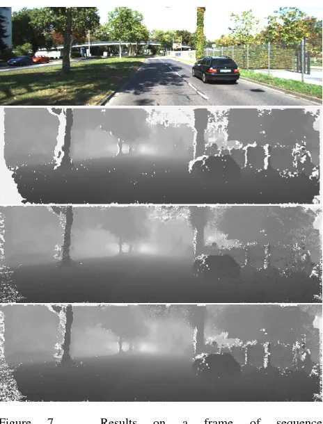
Color information provides the RGDF algorithm with a very sen-sitive means for distinguishing samples belonging to different ob-jects. Thus it is unsurprising that in spite of the fact that RGBF assumes scenes to be static, it handles scenes with moving objects quite well, cf. e.g. figure 7. Note though that for moving objects, the averaging yields atemporal averagingwhich results in ob-jects moving away from the camera being estimated too near and objects advancing towards the camera being estimated too far. It is plausible that this effect can be cancelled by suitable modelling and averaging, e.g. using the regression computation discussed in section 3.4.
6. CONCLUSION
We developed a disparity fusion method which uses radiomet-ric (color) images together with externally supplied camera pose information to fuse disparity images. It uses the comparison of radiometric values to distinguish correct sample matches from incorrect matches. Since radiometric information is a power-ful means for distinguishing objects, it allows the method to en-hance disparity images in particular at object borders and to re-strict the influence of moving objects to the pixels occupied by
Figure 7. Results on a frame of sequence
2011_09_26_drive_0013 of the KITTI raw data recordings. See fig. 3 for parameter description. Note the moving vehicle.
these objects. In particalar for the basic variant of RGDF, the improvements for static scenes are consistent over a large range of parameters. Furthermore, while outlier ratios are negatively affected by moving objects in a scene, they are virtually always better than the outlier ratios of the input data, which highlights the extreme robustness of the basic variant of RGDF. The algo-rithm is designed in such a way that most computations are simple and proceed virtually independent of each other, which facilitates parallelization and real-time performance even in simple imple-mentations. All in all, we obtain a computationally inexpensive algorithm which enhances edge quality drastically and which is robost enough to gracefully deal with moving objects.
REFERENCES
Chen, C., Cai, J., Zheng, J., Cham, T. J. and Shi, G., 2015. Kinect depth recovery using a color-guided, region-adaptive, and depth-selective framework. ACM Transactions on Intelligent Systems
and Technology (TIST)6(2), pp. 12.
Collins, R. T., 1996. A space-sweep approach to true multi-image matching. In: Computer Vision and Pattern Recognition, 1996. Proceedings CVPR’96, 1996 IEEE Computer Society Conference on, IEEE, pp. 358–363.
Furukawa, Y. and Ponce, J., 2010. Accurate, dense, and robust multiview stereopsis.Pattern Analysis and Machine Intelligence,
IEEE Transactions on32(8), pp. 1362–1376.
Gehrig, S. K., Eberli, F. and Meyer, T., 2009. A real-time low-power stereo vision engine using semi-global matching. In:
Com-puter Vision Systems, Springer, pp. 134–143.
Geiger, A., Lenz, P., Stiller, C. and Urtasun, R., 2013. Vi-sion meets robotics: The kitti dataset. International Journal of
SGM basic feedback
# IVs - 10 15 5
sequence nr.
0001 0.177 0.081 0.071 0.076
0002 0.178 0.083 0.073 0.076
0005 0.341 0.315 0.331 0.337
0009 0.269 0.193 0.191 0.195
0011 0.210 0.154 0.144 0.138
0013 0.312 0.224 0.229 0.225
0014 0.266 0.190 0.184 0.187
0017 0.231 0.228 0.223 0.235
0018 0.234 0.216 0.215 0.223
0019 0.235 0.154 0.152 0.159
0020 0.333 0.286 0.290 0.288
0022 0.262 0.229 0.237 0.234
0023 0.292 0.233 0.232 0.234
0035 0.213 0.170 0.170 0.163
0036 0.275 0.204 0.200 0.206
0039 0.260 0.188 0.188 0.199
0046 0.245 0.241 0.252 0.294
0048 0.251 0.172 0.171 0.182
0051 0.256 0.188 0.190 0.186
0056 0.204 0.129 0.159 0.161
0057 0.312 0.297 0.305 0.325
0059 0.280 0.255 0.264 0.287
0060 0.222 0.211 0.206 0.216
0091 0.283 0.189 0.186 0.196
0104 0.327 0.252 0.239 0.245
0106 0.324 0.275 0.280 0.302
0113 0.408 0.336 0.334 0.338
0117 0.307 0.270 0.279 0.279
Table 8. Outlier ratios for select sequences of the KITTI raw data recordings. The sequences used are 2011_09_26_drive_xyzw, with the sequence number xyzw given above. All RGDF vari-ants use a color dissimilarity threshold of 0.1.
Hilton, A., Stoddart, A. J., Illingworth, J. and Windeatt, T., 1996. Reliable surface reconstruction from multiple range images. In:
Computer Vision—ECCV’96, Springer, pp. 117–126.
Hirschmüller, H., 2005. Accurate and efficient stereo processing by semi-global matching and mutual information. In:Computer Vision and Pattern Recognition, 2005. CVPR 2005. IEEE
Com-puter Society Conference on, Vol. 2, IEEE, pp. 807–814.
Kenney, J. and Keeping, E., 1962. Linear regression and correla-tion.Mathematics of statistics1, pp. 252–285.
Liu, S., Lai, P., Tian, D., Gomila, C. and Chen, C. W., 2010. Joint trilateral filtering for depth map compression. In:Visual
Commu-nications and Image Processing 2010, Vol. 7744, International
Society for Optics and Photonics, pp. 77440F–77440F–10.
Liu, Y., Cao, X., Dai, Q. and Xu, W., 2009. Continuous depth estimation for multi-view stereo. In: Computer Vision and
Pat-tern Recognition, 2009. CVPR 2009. IEEE Conference on, IEEE,
pp. 2121–2128.
Menze, M. and Geiger, A., 2015. Object scene flow for au-tonomous vehicles. In:Proceedings of the IEEE Conference on
Computer Vision and Pattern Recognition, pp. 3061–3070.
Merrell, P., Akbarzadeh, A., Wang, L., Mordohai, P., Frahm, J.-M., Yang, R., Nistér, D. and Pollefeys, J.-M., 2007. Real-time visibility-based fusion of depth maps. In: Computer Vision,
2007. ICCV 2007. IEEE 11th International Conference on, IEEE,
pp. 1–8.
Pock, T., Zebedin, L. and Bischof, H., 2011. Rainbow of
Com-puter Science. Springer Berlin Heidelberg, chapter TGV-fusion,
pp. 245–258.
Rothermel, M., Wenzel, K., Fritsch, D. and Haala, N., 2012. Sure: Photogrammetric surface reconstruction from imagery. In:
Proceedings LC3D Workshop, Berlin, Vol. 8, pp. 1–9.
Rumpler, M., Irschara, A. and Bischof, H., 2011. Multi-view stereo: Redundancy benefits for 3d reconstruction. In: 35th
Workshop of the Austrian Association for Pattern Recognition,
Vol. 4.
Rumpler, M., Wendel, A. and Bischof, H., 2013. Probabilistic range image integration for dsm and true-orthophoto generation.
In:Image Analysis, Springer, pp. 533–544.
Schmeing, M. and Jiang, X., 2013. Color segmentation based depth image filtering. In:Advances in Depth Image Analysis and
Applications, Springer, pp. 68–77.
Sibley, G., 2007. Long range stereo data-fusion from moving platforms. PhD thesis, University of Southern California.
Tagscherer, R., 2014. Entwicklung und Test von 3D gestützten Verfahren für ein Augmented Reality System im Fahrzeug. Bach-elor’s thesis, Duale Hochschule Baden-Württemberg.
Toldo, R., Fantini, F., Giona, L., Fantoni, S. and Fusiello, A., 2013. Accurate multiview stereo reconstruction with fast vis-ibility integration and tight disparity bounding. International Archives of Photogrammetry, Remote Sensing and Spatial
Infor-mation Sciences40(5/W1), pp. 243–249.
Unger, C., Wahl, E., Sturm, P., Ilic, S. et al., 2010. Probabilistic disparity fusion for real-time motion-stereo. In: Asian
Confer-ence on Computer Vision (ACCV), Citeseer.
Wheeler, M. D., Sato, Y. and Ikeuchi, K., 1998. Consensus sur-faces for modeling 3d objects from multiple range images. In:
Computer Vision, 1998. Sixth International Conference on, IEEE,
pp. 917–924.