ANALYSIS OF THE EFFECT OF WAVE PATTERNS ON REFRACTION
IN AIRBORNE LIDAR BATHYMETRY
P. Westfelda,∗, K. Richtera, H.-G. Maasaand Robert Weißb
a
Institute of Photogrammetry and Remote Sensing, Technische Universit¨at Dresden, D01062 Dresden, Germany -(patrick.westfeld,katja.richter1,hans-gerd.maas)@tu-dresden.de
b
German Federal Institute of Hydrology, D-56068 Koblenz - [email protected]
Commission I, WG I/2
KEY WORDS:Airborne LiDAR bathymetry, multimedia photogrammetry, refraction, wave pattern, accuracy analysis
ABSTRACT:
This contribution investigates the effects of wave patterns on 3D point coordinate accuracy in LiDAR bathymetry. The finite diameter refracted laser pulse path passing the air/water interface is modelled differentially and in a strict manner. Typical wave patterns are simulated and their impact on the 3D coordinates at the bottom of the water body are analysed. It can be shown that the effects of waves within small LiDAR bathymetry footprints on the depth and planimetry coordinates is significant. Planimetric effects may reach several decimetres or even metres, and depth coordinate errors also reach several decimetres, even in case of horizontal water body bottom. The simplified assumption of averaging wave effects often made in many ALB applications is not only fulfilled in cases of a very large beam divergence under certain wave pattern conditions. Modern smaller beam divergence systems will mostly experience significant wave pattern dependent coordinate errors. The results presented here thus form a basis for a more strict coordinate correction if the wave pattern can be modelled from the LiDAR bathymetry water surface reflections or other observations. Moreover, it will be shown that the induced coordinate errors contain systematic parts in addition to the local wave surface dependent quasi-random part, which allows for the formulation of wave pattern type dependent correction terms.
1. INTRODUCTION
Airborne LiDAR bathymetry (ALB) is a technique to derive the underwater topography by airborne laser scanning, provided shal-low water areas and sufficient water transparency (e. g. Irish and Lillycrop, 1999; G¨unther, 2000). The technique captures both the surface as well as the bottom of the water body by scanning with green or red and green laser wave lengths simultaneously. ALB is recently gaining much attention due to new sensor develop-ments allowing for a much higher spatial resolution in scanning riverbeds and also due to EU regulations requiring hydrographic measurements in water bodies at regular time intervals (Mandl-burger et al., 2011).
Geometric modelling in airborne LiDAR bathymetry is more complex than in conventional laser scanning. Refraction effects of the laser pulse passing the air/water and water/air interfaces have to be taken into consideration. This includes the consider-ation of the reduced velocity of light in water (≈225 000 km/s) and geometric effects of multimedia photogrammetry (e. g. Maas, 2015). The simplest method is assuming a horizontal planar wa-ter surface at which the laser beam is refracted on the basis of Snells law. However, even small deviations from the planarity lead to significant measurements errors. Strictly speaking, the local wave-induced water surface inclination needs to be known for every single laser beam. Otherwise wave movements lead to a geometric displacement of the point hit at the bottom of the wa-ter body. This effect can take significant dimensions in the mewa-ter range, depending on water depth and wave parameters.
Many of the early airborne bathymetric LiDAR sensor systems operate with a large beam divergence of typically up to 21 mrad (G¨unther, 1985). The diameter of such a beam profile can eas-ily amount to several meters on the water surface. This ‘large
∗Corresponding author
footprint’ will often cover multiple wave cycles and is therefore considered to justify the assumption that wave effects are aver-aged. The situation for recent high resolution LiDAR bathymetry systems is rather different. Together with much higher pulse rates, they use low-divergence laser beams (‘small footprint’, e. g. 0.7 mrad) which requires new concepts of geometric modelling, as the effects of waves on the water surface cannot be neglected anymore when modelling refraction.
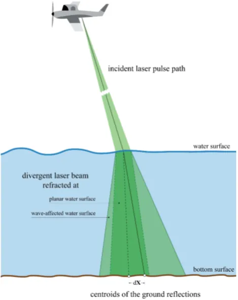
The aim of the paper presented here is to investigate the effect of waves on the water surface on the refraction affecting the path of the laser pulse under water (Figure 1). Typical wave patterns are simulated and their impact on the 3D coordinates (both depth and planimetry) at the bottom of the water body are analysed. The laser beam is not treated as an infinitesimal small line but passes the air/water interface with a finite cross section. Depending on the intensity distribution within this cross section as well as on the inclinations of the corresponding water surface elements, the refraction of the laser ray path is modelled differentially and in a strict manner.
The models developed can be used in two ways: If the actual water surface is known (for instance from dense laser scanner points representing the water surface or from image reflection based methods), each laser pulse may be corrected. If this infor-mation is not given, average effects may be calculated by simula-tions and applied as a correction term covering systematic effects introduced by wave patterns. This paper will focus on the latter aspect, showing that waves on the water surface have a signif-icant systematic effect on the bottom coordinates. That means that the accuracy of LiDAR bathymetry can significantly be im-proved when applying correction terms, which can be obtained by simulations for typical wave patterns.
Figure 1: Effects of wave patterns on 3D point coordinates.
Section 2. In Section 3, the results achieved are presented. Sec-tion 4 finally summarises the work and addresses future tasks.
2. METHODOLOGY
ALB measurements are characterized by the refraction of the laser ray passing the air/water interface and by an increased dis-persion of the laser pulse under water (G¨unther, 1985). Both ef-fects cause geometric displacements of the bottom points as well as a degradation of the optical signal which cannot be neglected anymore.
This contribution focusses on modelling effects of waves on the water surface on refraction. The effect of signal loss caused by turbidity is treated in (Richter et al., 2016).
Refraction effects on the optical path can be modelled by Snell’s law:
In the case of ALB applications, the laser pulse is travelling from air with a refractive indexn1 of near to1.0into the water body with a refractive indexn2of ca. 1.33(depending on water tem-perature, depth and salinity; see H¨ohle, 1971). After passing the media interface with an incident angleα1, the optical path is re-fracted towards the surface normal and the laser light is slowed down (v2 < v1). The procedure is the same for the reflected pulse with the laser light travelling from water to air refracted away from the surface normal.
It is obvious that deviations from planarity at the air/water inter-face will lead to variations in the surinter-face normal vector. These variations directly translate into errors in the local refraction an-gle and thus lead to 3D object coordinate errors at the water
bot-tom. The size of this error depends on the local surface inclina-tion at each 3D point of intersecinclina-tion and increase linearly with respect to the depth of the water.
Section 2.1 introduces the methods used for water surface simu-lations. Section 2.2 discusses the forward ray tracing (sensor→ air/water interface→water body bed).
2.1 Water Surface Modelling
Most ALB evaluation routines assume a planar water surface. This can be simulated by either a constant (mean) water level height over the entire area of investigation or by local horizon-tally oriented water surface elements at different heights. In the following analyses, local planar surface elements are compared to the non-planar water surfaces with wave patterns of varying com-plexity. The following formal descriptions of different types of waves were made in accordance to an oceanographics language (e. g. Holthuijsen, 2007).
Using periodic sine and cosine functions allows to model sim-ple symmetrical waves. The parameters amplitude and frequency specify the maximum height of a single wave as well as their width and maximum slope. Two types of wave patterns are anal-ysed (Table 1): Σ1 should correspond to slight, high frequency capillary waves such as they occur in a calm, rippled sea state (width: 37 cm; height: ±10 cm; slope: max. 30◦)1
. Σ2 should characterize a moderate sea state with long wind waves (width: 4 m; height:±1 m; slope: max. 25◦).
More complex, realistic sea swell simulations can be reached if horizontally and vertically running waves are modelled. Tessendorf’s (2001) algorithm for simulating ocean water orig-inates from computer graphics and is subjecting to an close to reality oceangraphic concept. The approach bases on a statistical model in which each wave height is a random variable of its lat-eral position and time. It decomposes the wave height field into a set of periodic waves with different amplitudes and phases. In-verse fast Fourier transform (IFFT) is finally used to evaluate the sum of these waves. Generating a random wave height field can be regulated by various parameters: The width, the height and the mesh size of the Fourier grid take influence on the dimension of the waves as well as on the level of detail. Further, the wind speed, which influences the largest possible waves arising, and the direction of the wind can be stated. A numeric constant is responsible for model scaling.
Three types of wave patterns are treated for complex modelling (Table 1):Υ1should represent a calm, rippled sea with short but steep waves and is thus comparable toΣ1 (average distance be-tween local minima and maxima: 10 cm; height: ±5 cm; slope: max. 65◦). Smooth, shallow wavelets with small crests and troughs should be modelled byΥ2(average distance between lo-cal minima and maxima: 50 cm; height: ±15 cm; slope: max. 25◦). InΥ
3, a water surface with moderate wave heights and long sea swell comparable to Σ2 should be simulated (average dis-tance between local minima and maxima: 6 m; height: ±1.5 m; slope: max. 45◦).
In the simulations based on these models, a 3D regular grid with a predefined mesh size of 20 mm×20 mm defines the topogra-phy of the water surface (X Y). Both parametric modelsΣand
1
The following conventions are made to quantify the wave patterns simulated: The maximum deflection in±Zis termed aswave height.
Periodic wave patterns
Σ1 Σ2
Slight, high frequency capillary waves (rippled sea).
Moderate, long ocean waves.
Complex wave patterns
Υ1 Υ2 Υ3
Short, smooth swell (rippled sea). Shallow waves with small crests and troughs.
Moderate, long ocean waves.
Table 1: Level of complexity in water surface modelling: The effects of water surface inclination on bottom point determination are analysed for periodic (Σ) as well as complex wave structures (Υ).
(a) (b)
Υare then used to generate the height field (Z) for the waves. The mesh size at the 3D water bottom grid is 80 mm×80 mm which turned out to be sufficient for a relatively smooth, contin-uous topology (Figure 2). Bicubic interpolation on the air/water resp. water/bottom interface grids approximates the value for the desired intersection points.
2.2 Ray Path Modelling
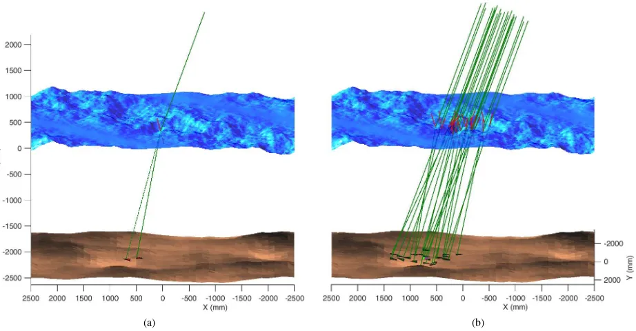
A first (simple) level of complexity treats the laser pulse as an in-finitesimal small line (Figure 2a). Obeying to Snells Law (Equa-tion 1), the laser light is refracted on its forward path once at an inclined water surface. The effect of wave patterns is already clearly recognisable but tends to be more distinct due to the sim-plified assumption of an infinitesimal small laser footprint fully subjected to any local surface inclination.
To get closer to the real situation, the laser light should pass the air/water interface with a finite cross section, necessitating differ-ential modelling of each infinitesimal refracted laser pulse path (Figure 2b). The intensity distribution within the incident laser pulse should follow a Gaussian intensity profile. The irradiance
Iis symmetric about the pulse axis (I=100 %) and varies with a radial distancer till the outer profile is reached atr = rmax
havingI=e−2
=13.5 %:
I(r) =I0·e2 r2/r2
max (2)
For further analysis, the resulting ground reflections are repre-sented by centroid coordinates, weighted accordingly to this in-tensity distribution.
3. RESULTS
The following Section 3.1 analyses the effect of wave patterns on the refraction of the path of the finite diameter laser pulse under water and the impact on the 3D coordinates. Section 3.2 asso-ciates changes in laser footprint’s size and shape with this effect.
Five typical sea swells at two different complexity levels were simulated at 100 consecutive epochs each. For computational is-sues, the number of infinitesimal paths representing a finite cross section was set to 50. Further relevant parameters are defined with respect to an airborne survey campaign conducted in 2014, where a Leica AHAB ChiropteraILiDAR system was used (Weiß, 2015): A flying height of 300 m and a beam divergence of 3 mrad allows for a relatively small laser footprint having an elliptic di-ameter of approximately 1 m at the water surface. The beam de-flection in the elliptical scanning pattern is 20◦.
As the effect of wave patterns on refraction increases linearly with the water depth, all results are presented as percentage of the water depth.
3.1 Coordinate Displacement
The geometric displacement of the point hit at the bottom of the water body consists of both a lateral component dX Y and a depth component dZ. Lateral displacements are caused by errors in the local refraction angle. They propagate as depth error, expressed as changes in ray path lengths, even if the water bottom is hori-zontal. The water body bottom topography additionally increases the effect.
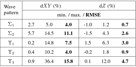
Table 2 summarizes the most important results for evaluating 3D coordinate displacements caused by non-modelled wave effects
on the differentially modelled laser ray paths. Here, the lateral coordinate displacement dX Y is calculated from the planimet-ric difference between the irradiance-weighted centroids of the ground reflections after refractions at wave-affected resp. hori-zontally oriented water surface elements. The underwater lengths of each refracted laser pulse path are calculated with respect to its intensity distribution within the laser pulse cross section. The resulting differences dZin length between inclined and horizon-tally oriented water surface elements are further shown in Table 2. Note that this is a purely geometric consideration of the effect of wave patterns on divergent laser pulses, which will in prac-tice also be affected by the obtained signal waveforms and their processing.
Table 2: Planimetric and depth coordinate displacement (in per-cent of water depth).
For the simulation at hand, a relatively large ‘small footprint’ of 3 mrad was used. All effects will further increase for recent LiDAR systems operating with narrower beam divergences (for instance 0.7 mrad for the RIEGL VQ-880-G).
In the following, the lateral effects are discussed first, followed by the depth errors.
The rather simple periodic wave patterns Σare analysed first. The root mean square error (RMSE) of the lateral displacement can be estimated to be 4 % of the water depth for the sea swellΣ1 and 11 % forΣ2(Table 2, row 1–2). It already becomes obvious at this stage that wave effects do not average out. In fact, sig-nificant systematic effects remain. Even if multiple wave cycles are within the laser footprint, the common assumption made in many ALB applications cannot be taken for granted. Further, the effect of local wave inclination on refraction is increasing with increasing period length and constant slope (wave period>laser footprint).
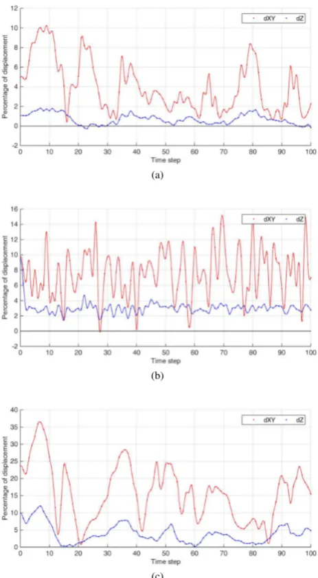
The RMSE of the lateral coordinate displacements dX Y is 7.5 % (max. 14.8 %) for the smooth, rippled sea swellΥ1 (Table 2, row 3; Figure 3a). Assuming a mean water depth of 5 m leads to a RMSE of 40 cm (max. 74 cm). The longer but less steeply running shallow sea swellΥ2results in a RMSE of 4.0 % (max. 10.2 %), which corresponds to 20 cm (max. 51 cm) in 5 m wa-ter depth (Table 2, row 4; Figure 3b). Using more complex pat-terns for wave simulation confirms the evaluation stated above that multiple wave cycles do not completely average out over the laser footprint area. The laser beam deflection as well as a turbu-lent, chaotic sea swell increase the effect additionally.
meters underwater. Again this clearly manifest that shifting ef-fects induced by local wave inclination are more distinct if water waves with period lengths greater than the size of the laser foot-print are permeated.
(a)
(b)
(c)
Figure 3: Percentage of coordinate displacement depending on water depth for (a) sea swell Υ1 (dX Y=7.5 %, max. 14.8 %; dZ=3.0 %, max. 6.3 %), (b) sea swell Υ2 (dX Y=4.0 %, max. 10.2 %; dZ=0.7 %, max. 1.8 %) and (c) sea swell Υ3 (dX Y=15.8 %, max. 36.4 %; dZ=3.9 %, max. 12.0 %).
The coordinate errors obtained for the more realistic modelled sea swellΥ1are comparable to the straightforward simulated sea swellΣ1, both representing small ripples on a rather smooth sea. The ocean waterΥ3corresponds approximately toΣ2. The anal-yses of the lateral displacement vectors have clearly shown that improvements in 3D object coordinate determination can already be achieved if the water surface is modelled by simple symmetri-cal waves. For the simulations at hand, the use of more complex, asymmetric-wave models increases these improvements by a fac-tor 2.
The lateral displacement stated above propagates as depth error. In order to evaluate changes in pulse travel time, the underwa-ter lengths of each refracted laser pulse path are calculated with
respect to its intensity distribution within the laser pulse cross section. The differences dZin length between inclined and hor-izontally oriented water surface elements are shown in Table 2 and as blue curves in Figure 3.
In conclusion, RMS depth errors in the range of 0.9 % to 4.7 % can be expected for the complex modelled sea statesΥ(Table 2, row 3–4. last column; Figure 3). Assuming a mean water depth of 5 m, this corresponds to 45 mm to 235 mm, with max-ima reaching 12.0 % (0.6 m at 5 m water depth). Apart from a few exceptions, the underwater laser ray path becomes longer for wavy water surfaces. The transit time registered at the sensor is therefore too long, and the water body bottom model calculated becomes too deep.
Strictly applying corrections for compensating these planimetry and depth coordinate errors requires high resolution models of the instantaneous water surface. These models may basically be derived from LiDAR bathymetry water surface points. In many applications, however, the point density will not be sufficient to model complex wave patterns on the water surface. In these cases, the simulations shown above may form a basis to derive correction terms for typical wave patterns, which can be applied to the water body bottom coordinates in order to at least partly correct for the wave induced errors.
3.2 Laser Footprint
Wave effects will also influence the size and the shape of the laser pulse under water. In order to investigate those changes, the laser footprint at the water surface is compared to the underwater foot-print at the bottom.
For each time step, an ellipse was fitted into the outer points of the differentially modelled laser footprint at the water surface (Fig-ure 4a). The length of the major resp. minor axis provide suit-able information on laser footprint dimension. Due to local wave-induced water surface inclination, the underwater laser footprint appears rather blurred. The simulated discrete points forming the laser footprint are misaligned (Figure 4b), and the intensity dis-tribution no longer follows a Gaussian disdis-tribution (Figure 4c vs. 4d). An ellipse fit is thus not suitable to quantify the size of a footprint at the bottom. Alternatively, the first and second prin-cipal component as result of a prinprin-cipal component analysis are intersected with the outer shell of the laser footprint polygon.
The differences between the first principal component and the major axis resp. the second principal component and the minor axis are listed in Table 3. The laser footprint is subject to changes of its size inX- andY-direction, depending on the length and orientation of the wave exposed to laser light as well as on the flight and scan direction. Here both beam expansion and beam focussing may occur, but in average most of them are expanded.
Considering for example the calm, ripple sea stateΥ1, the laser beam transmitted from an altitude of 300 m, originally having an almost elliptically shape of ca. 95 cm×101 cm at the water sur-face, expands by in average 1.6 m in the direction of the major axis to more than 2.5 m in 5 m water depth. A slight focussing of in average 23 cm occurs in the direction of the minor axis. Please note that all values stated above include an expansion of 3 mm/m caused by beam divergence.
4. SUMMARY AND OUTLOOK
(a) (b)
(c) (d)
Figure 4: Wave-induced changes in laser beam’s size and shape: (a,c) Laser footprint at the water surfaceΥ1; 959 mm×1010 mm; almost ideal Gaussian intensity profile. (b,d) Laser footprint at the water bottom in 1 metre depth; 1403 mm×1180 mm; irregular intensity distribution.
Wave pattern
1stPC – MajAx (%)
2ndPC – MinAx (%)
min. / max. /mean
Υ1 -0.5 74.9 32.4 -27.4 22.1 -4.6
Υ2 -15.5 57.3 7.6 -34.6 8.0 -9.9
Υ3 17.4 79.6 43.9 -0.5 42.7 21.0
Table 3: Change in laser footprint size specified as difference be-tween the first principal component (1stPC) and the ellipse major axis (MajAx) resp. the second principal component (2ndPC) and the ellipse minor axis (MinAx) (in percent of water depth).
and their impact on the 3D coordinates at the bottom of the wa-ter body were analysed. It has been shown that, depending on water depth and wave heights, the effect on lateral bottom point displacement can take on significant dimensions in the range of several decimetres, in some cases even several metres. Further-more, local depth errors in decimetre range have to be taken into consideration. The simplified assumption of averaging wave ef-fects often made in many (large foortprint) ALB applications is not fulfilled. The effect scales up for modern LiDAR bathymetry systems, which came with much smaller footprints and cannot be neglected in most situations.
There are basically two methods for reducing these coordinate
errors: A strict procedure would require modelling the instanta-neous water surface in order to perform a strict differential ray tracing for each laser pulse. This will often not be possible due to insufficient information for instantaneous water surface mod-elling. As an alternative, correction terms may be applied for typical wave patterns, which may be derived from the simulations shown in the paper.
Future work will concentrate on more extensive simulations con-sidering dependencies on beam divergence, beam deflection and aircraft altitude. In a next step, local wave patterns should be modelled on the basis of real LiDAR bathymetry water surface reflections or other observations. As final result, more strict co-ordinate correction terms can be applied in order to increase the accuracy potential of applications in airborne LiDAR bathymetry.
References
G¨unther, G. C., 1985. Airborne laser hydrography system de-sign and performance factors. Rockville, Md.: U.S. Dept. of Commerce, National Oceanic and Atmospheric Administra-tion, National Ocean Service, Charting and Geodetic Services.
H¨ohle, J., 1971. Zur Theorie und Praxis der Unterwasser-Photogrammetrie. Bayerische Akademie der Wissenschaften (M¨unchen). Deutsche Geod¨atische Kommission. Reihe C, Beck.
Holthuijsen, L. H., 2007. Waves in Oceanic and Coastal Waters. Cambridge University Press. Cambridge Books Online.
Irish, J. L. and Lillycrop, W., 1999. Scanning laser mapping of the coastal zone: the SHOALS system. ISPRS Journal of Pho-togrammetry and Remote Sensing 54(23), pp. 123 – 129.
Maas, H.-G., 2015. On the accuracy potential in underwa-ter/multimedia photogrammetry. Sensors 15(8), pp. 18140.
Mandlburger, G., Pfennigbauer, M., Steinbacher, F. and Pfeifer, N., 2011. Airborne hydrographic LiDAR mapping - poten-tial of a new technique for capturing shallow water bodies. In: Modelling and Simulation Society of Australia and New Zealand, Perth, Australia, pp. 2416–2422.
Richter, K., Westfeld, P., Maas, H.-G. and Weiß, R., 2016. Korrektur der Signald¨ampfung und Analyse zur Bestimm-barkeit der Gew¨assertr¨ubung in Laserbathymetrie-Daten. In: Dreil¨andertagung D-A-CH der DGPF, OVG und SGPF, Bern, CH.
Tessendorf, J., 2001. Simulating ocean waters. In: ACM SIG-Graph Course Notes, Vol. 47.