DETECTION OF ROAD CURB FROM MOBILE TERRESTRIAL LASER SCANNER
POINT CLOUD
Sherif El-Halawany *, Adel Moussa, Derek D. Lichti and Naser El-Sheimy
Department of Geomatics Engineering, University of Calgary, Canada
(smmibrah, amelsaye, ddlichti, elsheimy @ucalgary.ca)
Commission V, WG V/3
KEY WORDS: road furniture, curb, street floor, sidewalk, eigenvalue, surface normal, edge detection
ABSTRACT:
The detection of different road furniture such as curb, street floor and sidewalk from point clouds is important in many applications such as road maintenance and city planning. In this paper a pipeline for point cloud processing to detect the road curb from unorganized point clouds captured from a mobile terrestrial laser scanner is proposed. The proposed pipeline utilizes a covariance-based procedure to perform a 3D segmentation of point clouds. Features such as the road curb can be extracted by analyzing the local neighborhood of every point. This is done by computing the surface normal direction and the normalized eigenvalues. These parameters can be used to extract the ground objects, such as curb, street floor and sidewalk. The curb can be isolated from the rest of the ground objects based on the previous parameters in addition to elevation gradient within the local neighborhood. A 2D image processing scheme is also presented to find the curbs as edges in a generated 2D height image. The results show successful detection rates of 78% and 94% using 3D and 2D approaches respectively.
* Corresponding author.
1. INTRODUCTION
The market is seeing a rapid growth in utilizing the mobile laser scanning (MLS) systems in many road corridors applications. There are many systems all around the world such as, TITAN, StreetMapper, and RIEGL VMX-250. These systems are fast and more accurate; which allow a very high dens point clouds to be acquired. But their use is still limited due to their cost and the huge amount of data they capture. It is important to automate the detection of road features such as road curb from the point cloud captured by these systems.
Road curb represents a very important part of the road. It separates the street floor and side walk and is used to direct rainwater into the drainage system. The aim of this research is to automatically identify the road curb from an unorganized 3D point cloud of a road scene; the data have been captured by a vehicle-based laser scanning system named TITAN.
2. LITERATURE REVIEW
Research has been aimed at reducing the cost of the point cloud processing by automating part of the processing, namely the extraction of road curb and isolating surrounding geometric features like poles. Belton and Bae (2010) proposed a method to extract the 2D cross section of the curb, where the curb profile can be analyzed to segment curb features, such as poles and signs. First, they stored the point cloud in a 2D grid, and extracted the road surface by selecting the lowest points in height in each grid cell. Then they extracted the different objects close to the road surface, such as road curb. The curb line is extracted by fitting a curb profile and joining adjacent profiles to form a linerepresentation of the curb.
There are two main limitations for the proposed method by Belton and Bae. First, they assumed that the ground points are located on the lowest, smooth, horizontal surface; this assumption is not always true especially in roads which have under passes. Second, identifying the road surface based on the lowest points in height in each grid cell and fitting a curb profile will not always work with MLS data, where MLS data have a different nature compared to data captured by stationary scanning. MLS point cloud suffers many problems such as, data artefacts, combination of multiple data sources, and mis-registering of multiples drivelines. There is a need for new techniques for curb extraction from MLS data.
A recent approach applied with point clouds captured by a mobile TLS from moving platforms analyzes the cross section profile by the laser range points (Chen et al., 2007). The road boundary can be detected by analyzing the cross sections profiled by laser range points. Because the road surface appears as a straight line in the scan, the longest straight line in one scan line can be chosen in order to extract the road boundary. New methods are needed because the available data in this study are unorganized 3D point clouds that do not have profile information.
Jaakkola et al. (2008) developed a method for identifying the road curb from MLS point clouds. This method applies 2D image processing techniques on intensity and height images. These images are used to detect the curb stones. They applied this method on a short road sample with a straight curb in one extension, where the street direction is known. The available data in this paper have varieties of road curbs, with different shapes (straight and curved) and extensions (North-South and East-West).
3. STUDY AREA AND DATA
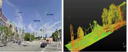
The used data in this study was captured by TITAN. TITAN is a mobile laser scanning system for highway corridor surveys; it can be deployed on a passenger vehicle or small watercraft, (Figure 1). Light detection and ranging (LiDAR) digital imagery and video data are collected from the survey platform while it is moving at traffic speeds. The system is georeferenced with a high accuracy Global Positioning System (GPS) – Inertial Measurement Unit (IMU), (Glennie, 2008). The data represent part of Elgin Street in the downtown of Ottawa city (Figure 2, left). The number of points is ~ 5 million and the point cloud density is ~ 400 pt/m2
on the street floor. The size of the point cloud ( x, y, z) is approximately (106.0m, 98.0m, 34.0m).
Figure 1. TITAN mobile laser scanning system. Left: Close view. Right: Mounted on a truck.
www.ambercore.com
This part of Elgin Street has been chosen because it has an intersection, straight and curved curbs, and many pedestrian sidewalks, which makes the extraction of the curbs more complicated. Figure 2, right, represents the input point clouds before performing the curb segmentation.
Figure 2. Part of Elgin Street, Ottawa. Left: Google maps (street view). Right: 3D point clouds.
4. PROPOSED METHODOLOGY
The pipeline of the curb extraction consists of 5 phases. In the first phase the input 3D point cloud of the road scene is organized and then the principal components analysis (PCA) is performed. The second phase aims at segmenting the point cloud into two main segments; the first one is the ground while the second is non-ground. Furthermore, the ground segment is refined in the third phase in order to get rid of some non-ground objects such as parts of trees, poles and buildings. The fourth phase extracts just the curb boundaries, street floor and the side walk from the refined ground segment. Finally, the fifth phase isolates the curb from the street floor and sidewalks by using 3D and 2D techniques. In order to implement the different processing steps within the different phases, a C++ program has been built using Visual Studio 2008.
4.1 First Phase
Because the input is an unorganized 3D point cloud, the pipeline of this research starts with organizing the point cloud by utilizing a data structure technique such as the well known neighborhood search step, every point will form a cluster with its spherical neighbor points, from which we can compute the covariance matrix (C) for each cluster by using Equation 1.
where k is the number of k-nearest neighbors at a query point,
i
r
is the position vector of point i and r is the mean position (centroid) for the cluster. The covariance matrix is a 3x3, real, positive, semi-definite matrix, the eigenvalues of which are always greater than or equal to zero. The eigenvalues (λs) can be examined to detect points with a certain structure, such as planar features in the neighborhood, (Kukko et al., 2009; Briese and Pfeifer, 2008). The relative sizes of the eigenvalues and the eigenvector directions can indicate the type of primitive feature, (Gross and Thoennessen, 2006); where the point cloud can be classified into main groups such as linear and planar features, (Belton and Lichti, 2006). For a planar feature there are two almost equal and one small normalized eigenvalues. The three eigenvalues obtained from PCA can be reordered to adopt theThe input point cloud is segmented into two main segments, the first one is the ground while the second is non-ground. Figure 3 demonstrates the different processing steps for both the first and second phases. The segmentation is done based on the relative sizes of the normalized eigenvalues and the surface normal direction. The surface normal is defined as the eigenvector of the smallest eigenvalue, which can be obtained from the eigenvalue decomposition (Equation 3), where
e
1,e
2 and3
e are the three eigenvectors of the eigenvalues respectively.
(
)
Figure 3. Pipeline of the first and second phases.
Figure 4 shows the surface normal directions for different objects in a road cross section. The surface normal makes an angle of 90o with the horizontal plane for objects such as street floor, side walk, building rooftops. On the other hand, objects like poles, building facades, tree foliage and curb have different surface normal direction inclinations with the horizontal plane. The ground can be segmented by labelling all points which have an approximately vertical surface normal direction and planar neighborhoods.
Figure 4. Surface normal direction for a road cross section.
The extracted ground segment will include all planar objects such as, street floor, sidewalk, curb boundaries, side gardens and building roof tops. Table 1 lists the different parameters which have been used for segmenting the ground from the input point cloud as well as their thresholds. These thresholds have been defined based on the properties of the objects of interest; For example, the neighborhood size (k) and the search radius are defined based on the density of the point cloud.
Table 1. Thresholds of different parameters-second phase.
The thresholds for surface normal (θ) is between 81 o and 90o and for the three normalized eigenvalues are set to find all surfaces in the point cloud like street floor and side walk.
4.3 Third Phase
The segmented ground still has some parts of trees, poles and building facades which are missegmented as part of ground segment. The aim of the third phase is to refine out the extracted ground by removing those objects. This is done by
segmenting the ground based on recalculating the parameters and using the thresholds of Table 1.
4.4 Fourth Phase
By fitting a plane to the refined ground segment, objects like building roof tops and some areas which lie under the street level (underpass) can be removed from the ground segment. The equation of the principal plane can be formed based on the coordinates of the centroid (x0, y0, z0) and the normal to the plane (eigenvector of the smallest eigenvalue), Equation 4.
(4)
where a, b, c are the direction numbers for the normal to the plane (i.e. the eigenvector). The idea is to fit a plane to the ground segment and then compute the normal distance (d) for all points to that plan, (Equation 5), where x, y, z are the coordinates of the point. A threshold can be set to d in order to end up with just the street floor and the sidewalk. This is based on the assumption that the plane will fit most of the street floor points because this part of the data has the higher density.
(5)
Figure 5. Histogram of point to plane normal distance.
The histogram of d for all points above and below the fitted plane is presented in Figure 5. The point which has minimum d (normal distance to the plane) can be picked (point on plane), the elevation (Z coordinate) of this point will be used to define the elevation of the fitted plane (Zo). Then an elevation threshold can be set based on Zo. All points which have an elevation above or below Zo by specific thresholds will be removed from the ground segments. This leads to a filtered ground segment with only curb boundaries, street floor and sidewalk.
4.5 Fifth Phase
Finally, the boundary of the road curb can be extracted from the ground segment. Two different approaches have been tested; the first one is based on 3D analysis of the point cloud. The second approach is utilizing the 2D image processing techniques.
4.5.1 3D Approach
In this approach the curb is isolated based on the following parameters: the elevation gradient in the local neighborhood,
Parameter Threshold
No. points K=50
Search radius r = 0.1 m
Surface normal 90o > θ > 81o First normalized largest eigenvalue 0.63 >= Nλ1 > 0.4 Second normalized largest eigenvalue 0.6 >= Nλ2 > 0.3 Third normalized largest eigenvalue 0.1 >= Nλ3 > 0.0
0 = ) z -(z c + ) y -b(y + ) x
-a(x o o o
2 2 2
o) b( ) ( )] x
-abs[a(x d
c b a
z z c y
y o o
+ +
− + − + =
surface normal direction and the three normalized eigenvalues. A neighborhood for every point must have enough number of points in order to include point from different surfaces, where points lie on curb boundary are identified as those points which have difference in elevation greater than a specific threshold in their neighborhood. Table 2 gives the different thresholds which have been utilized to segment the curb boundaries from the street floor and sidewalk.
The thresholds for neighborhood size, search radius, surface normal direction, three normalized eigenvalues and the elevation gradient are defined based on the point cloud density as well as properties of the curb. Where a large values of K and r are chosen, to insure that the neighborhood will include points from the upper and lower boundaries of the curb. Because the curb boundary includes points from street floor and sidewalk, the surface normal direction will be shifted slightly from 90o, also the height of the curb is between 10 and 20 cm. The threshold for Nλ1 is set to detect edge features such as the curb boundaries.
Table 2. Thresholds of different parameters-fifth phase.
4.5.2 2D Approach
In this approach, the 2D height image which represents the point cloud is processed to detect the curbs instead of dealing with an irregular 3D point cloud. Two-dimensional processing enables the utilization of a wide variety of well established methodologies for 2D edge detection, and also decreases the computational effort due to the regular representation of data into a standard grid. The proposed 2D approach starts with gridding the point cloud into a regular lattice, then a standard edge detection technique is applied to find the curb candidates, finally the detected edges are filtered to remove the non curb edges.
As a first step, the 3D point cloud are projected onto the x-y plane and assigned to a lattice of adjacent squares covering the whole span of the data coordinates. The square size should be carefully chosen to be as small as possible while maintaining enough points to avoid getting too many empty squares. Based on the density of data points, the square size has been chosen to be 10 cm by 10 cm. The count and average height of the assigned points to each square represents the density and the height of this square respectively. The grid has been interpolated based on nearest neighbor to fill the empty entries. As curbs typically exhibit a sudden change in height, they can be detected using edge detection methodologies applied on the 2D height grid. In the proposed approach, Canny edge detection methodology has been chosen to extract the edges in the interpolated height profile. The Canny edge detection includes noise reduction using Gaussian filtering, computing the intensity gradient and finding the maximum localized edges, and finally tracing the detected edges to include the weaker
gradients if they exhibit natural extension to the strong edges (Canny, 1986). The former property of the Canny method helps to detect the weaker curbs typically found at the pedestrian crosswalks. The former step finds a lot of edges over the whole scanned scene besides the curb edges. These curb edges exist on the sides of the street floor which exhibits the highest point density across the whole scene. This high density is used in the proposed approach to filter out the non curb edges. The idea is to construct a mask to be used for rejection of non curb edges based on density.
5. RESULTS AND DISCUSSION
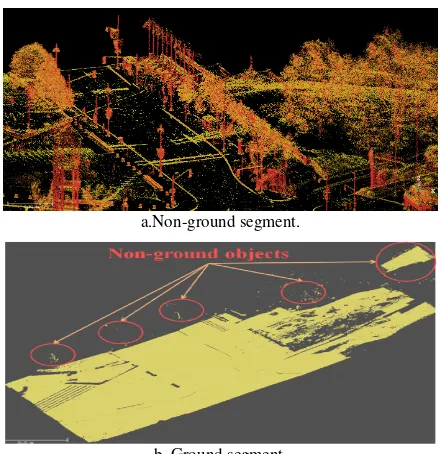
The 3D segmentation results for the second phase (Figure 6) are ground and non-ground segments. Figure 6.a shows the segmented non-ground objects, where most of the objects like poles, trees and buildings are successfully segmented as non-ground. On the other hand the ground segment (Figure 6.b) contains most of the objects which lie on the ground level, such as the street floor, sidewalk and curb boundaries. Due to data noise and non uniform distribution of the point cloud, the ground segment still contains some non-ground objects such as parts of poles and trees.
a.Non-ground segment.
b. Ground segment.
Figure 6. Segmentation result of the second phase.
The results obtained from the second phase can lead to different pipelines. For example, the ground segment is used in this study to extract the road curb; in addition, the street floor and sidewalk can be extracted from this segment too. On the other hand, the non-ground segment can be used as a preliminary step for the extraction of different objects like poles and trees, where extracting these objects becomes easier after removing the ground points. For example, the base of the poles can be fully extracted and will not be misidentified as planar features instead of linear ones as reported by El-Halawany and Lichti, 2011. This is due to removing the ground points surrounding the pole’s base (Figure 7). This will improve the result of any segmentation techniques, especially those relying on the neighborhood analysis of every point such as, the principal component analysis PCA.
Parameter Threshold
No. points K=500
Search radius r = 0.5 m
Elevation gradient 0.2 >= ∆z > 0.11 m Surface normal 87o >= θ > 83o First normalized largest eigenvalue 0.8 >= Nλ1 > 0.57 Second normalized largest eigenvalue 0.5 >= Nλ2 > 0.2 Third normalized largest eigenvalue 0.05 >= Nλ3 > 0.0
Figure 7. No ground points surrounding the poles’ bases.
Figures 8 left and right, show the extracted ground segment and the refined one from the second and third phases, it is clear that the segmentation parameters which have been used in phase three successfully refined the ground segment. The thresholds listed in Table 1 are close to the optimum ones, because they completely removed most of poles, trees, and building facades from the ground segment.
Figure 8. Segmentation results of third phase. Left: Unrefined ground segment. Right: Refined ground segment.
After the refinement, some non-ground objects are left over such as building rooftops and underpass, these objected are resulted from the segmentation of the second phase. These objects have the same values for the segmentation parameters as the ground objects have. For example, they have the same surface normal direction and normalized eigenvalues. Figures 9 and 10 compare the ground segment obtained from phase three (left images) and the one resulted from phase four (right images). It is clear that the point to plane normal distance-based filter successfully removed the non-ground objects such as the rooftops and underneath pass from the ground segments (regions surrounded by red circles). The used threshold for point to plane normal distance is 0.5 m. This threshold can be estimated based on the extension of the road and the elevation of the surrounding objects.
Figure 9. Segmentation results (top down view). Left: Ground segment-phase three. Right: Ground segment-phase four.
Figure 10. Segmentation results (side view). Left: Ground segment-phase three. Right: Ground segment-phase four.
Figure 11, left, illustrates the interpolated height profile, while Figure 11, right depicts the density of the data points in the same scanned area, where the density is computed as the number of points per grid.
Figure 11. Left: Height image. Right: Density image.
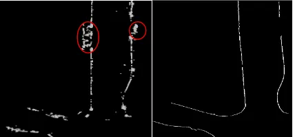
Figure 12 shows the detected edges of the interpolated height profile using the Canny method. The density profile depicted in Figure 12 cannot be used directly as it is in a discrete non-continuous form, therefore a median filtering of this density profile is first conducted to fill in gaps as illustrated in Figure 13, left.
Figure 12.The detected edges using Canny method.
The filtered density is then converted into a binary form to construct the required mask based on a density threshold as shown in Figure 13, right. Finally this mask is used to filter out the non curb edges as illustrated in Figure 14 right.
Figure 13. Left: The median filtered image. Right: The generated density mask.
Figure 14. The extracted road curb. Left: From 3D approach. Right: From 2D approach.
Figure 14 left shows the extracted road curb using 3D segmentation with the thresholds listed in Table 2, some parts are missing from the curb due to the presence of pedestrian cross walks. The results show some objects on the sidewalk like part of parked vehicles (surrounded by a red circles). It is hard to eliminate those objects because they are very close to the curb and have the same properties as the curb. Figure 14.b depicts the extracted road curb using 2D edge detection and filtration. The Canny edge detection helped to detect smooth linear curbs and to extend it along weaker regions of the pedestrian crosswalks. The non curb edges have been successfully removed using the density-based mask. The accuracy of the proposed curb detection methodologies were assessed with a reference data. This is done using a pixel-based comparison of the registered reference image and the detected curb image. The precision of the 3D approach achieved 83 %, while the recall was 78 %. On the other hand, the 2D approach achieved 97 % of precision, while the recall was 94 %.
6. CONCLUSION AND OUTLOOK
In this research a pipeline for curb segmentation from 3D unorganized point cloud has been proposed. The pipeline is split down into 5 main phases. First the point cloud is organized and the segmentation parameters are computed. Then, the point cloud is segmented into ground and non-ground based on the surface normal direction and the relative sizes of three normalized eigenvalues. After that, the segmented ground is refined out from unwanted objects such as parts of poles and trees. Furthermore, the building rooftops and underpass have been removed from the ground segment based on the normal distance to the plane threshold. Finally, the curb has been extracted using two different approaches based on 3D segmentation and 2D image processing methodologies respectively.
In the future, other data sets will be tested in order to evaluate the applicability of the proposed pipeline in detecting road curbs in different road scenes. Adding more information to the point cloud will be tested too. For example, the intensity information can be used to distinguish between the street surface and sidewalk. This can lead to better isolation of street floor from the obtained results of phase four. Future work will be focusing on how to automatically get the optimum thresholds for the different parameters, such as: neighborhood size, neighborhood search radius, three normalized eigenvalues, edge detection parameters, and the elevation gradient.
ACKNOWLDGEMENT
Thanks to the GEOmatics for Informed DEcisions (GEOIDE) network, Terrapoint Canada Inc. and Neptec Design Group Canada for their support, sponsoring this research and for providing the TITAN data.
REFERENCES
Belton D. and Bae K.-H., 2010. Automating post-processing of Terrestrial Laser Scanning point clouds for road feature surveys. Proceedings of ISPRS Commission V Mid-Term Symposium, Newcastle upon Tyne, UK.
Belton D., and Lichti D.D., 2006. Classification and segmentation of terrestrial laser scanner point clouds using local variance information. ISPRS Commission V Symposium 'Image Engineering and Vision Metrology'.
Briese, N. Pfeifer, 2008. Towards automatic feature line modelling from terrestrial laser scanner data. In Proceedings of the ISPRS XXIst Congress, Beijing, China, Vol. XXXVII. Part B5 (2008), ISSN: 1682-1750; 463 - 468.
Canny J., 1986. A computational approach to edge detection. IEEE Trans. Pattern Analysis Machine Intelligence, vol. PAMI-8, pp. 679-69PAMI-8, 1986.
Chen, Y.-Z., Zhao, H.-J., Shibasaki, R., 2007. A mobile system combining laser scanners and cameras for urban spatial objects extraction. Proceedings of the Sixth International Conference on Machine Learning and Cybernetics Hong Kong, vol. 3, pp. 1729 –1733, 19-22th August 2007.
El-Halawany S. and Lichti D.D., 2011. Detection of road poles from mobile Terrestrial Laser Scanner point cloud. International Workshop on Multi-Platform/Multi-Sensor Remote Sensing and Mapping, 10-12 January 2011, Xiamen, China.
Glennie, C. 2008. A kinematic terrestrial LiDAR scanning system. Transporation Research Board of the National Academies, In Press, Submitted: June 19, 2008.
Gross, H., Thoennessen, U., 2006. Extraction of lines from laser point clouds. In Symposium of ISPRS Commission III: Photogrammetric Computer Vision CV06. International Archives of Photogrammetry, Remote Sensing and Spatial Information Sciences 36 (Part 3), pp. 86-91.
Jaakkola, A., Hyyppä, J., Hyyppä, H., and A. Kukko, 2008. Retrieval algorithms for road surface modelling using laserbased mobile mapping. Sensors 8(9), pp. 5238-5249.
Kukko A., Jaakkola A., Lehtomäki M., Kaartinen H., Chen Y.,2009. Mobile mapping system and computing methods for modelling of road environment, Urban Remote Sensing Joint Event, 2009.
Mount, D.M. and Arya, S. ANN, 2006. A library for approximate nearest neighbor search, v.1.1.1, Aug.4, 2006 release. http://www.cs.umd.edu/~mount/ANN/.