Ž .
Atmospheric Research 55 2000 15–33
www.elsevier.comrlocateratmos
Microphysical properties of stratocumulus clouds
Hanna Pawlowska
a, J.L. Brenguier
b,), Frederic Burnet
ba
Institute of Geophysics, UniÕersity of Warsaw, Warsaw, Poland
b
Centre National de Recherches Meteorologiques, GMEI´ ´ rMNP, 42 aÕ. Coriolis,
31057 Toulouse Cedex 01, France
Received 11 December 1998; accepted 1 March 2000
Abstract
Data collected in situ with the Meteo-France Merlin-IV instrumented aircraft during the EUCREX mission 206 are analyzed to document cloud properties that are relevant to the calculation of cloud radiative properties. Ascents and descents through the cloud layer reveal that
Ž .
most of the vertical profiles of liquid water content LWC and droplet sizes are close to adiabatic profiles. Analysis of horizontal legs shows that sub-adiabatic regions are characterized by reduced droplet concentrations, while droplet sizes remain close to their adiabatic values at that level. Statistics of LWC, droplet concentration and droplet mean volume radius normalized by their adiabatic values are presented for four distinct regions of the cloud layer. This information is
provided for tests of a parameterization of optical thickness based on the adiabatic model.q2000
Elsevier Science B.V. All rights reserved.
Keywords: Cloud microphysics; Stratocumulus
1. Introduction
The radiative properties of warm clouds result from scattering of light by cloud droplets. They are thus modulated by the spatial and size distributions of the droplets, which are extremely variable. The challenge in the development of parameterizations of
Ž .
cloud radiative properties for general circulation models GCM is to express this
Ž
variability by a few parameters predictable at the GCM scale the typical grid of a GCM
.
is presently of the order 100–200 km .
)Corresponding author. Tel.:q33-5-61-07-93-21; fax:q33-5-61-07-96-27.
Ž .
E-mail address: [email protected] J.L. Brenguier .
0169-8095r00r$ - see front matterq2000 Elsevier Science B.V. All rights reserved.
Ž .
Ž .
Hansen and Travis 1974 have shown that the optical properties of a homogeneous cloud volume are expressed as functions of two microphysical variables: the liquid water
Ž .
content LWC and the droplet effective radius. In order to calculate the radiative transfer through a cloud, it is thus necessary to assume some spatial distribution of these parameters. An attractive simplification is to assume that the cloud is a horizontally infinite homogeneous layer of geometrical thickness H. This is referred to hereafter as
Ž .
the vertically uniform plane parallel model VUPPM . The two-stream approximation
ŽCoakley and Chylek, 1975; Stephens, 1978; Slingo, 1989 or the doubling–adding
´
.Ž .
matrix method Twomey et al., 1966 for radiative transfer calculations are based on this hypothesis. A vertically stratified cloud can then be modeled as a stack of VUPPMs
ŽSlingo and Schrecker, 1982 ..
Microphysical measurements in stratocumulus have revealed a significant variability
Ž
of LWC and effective radius in the horizontal as well as in the vertical Slingo et al.,
.
1982; Nicholls, 1984; Stephens and Platt, 1987; Martin et al., 1994 . The radiative transfer calculation is an integral over the cloud thickness and the vertical variability of
Ž .
the microphysics affects this integral in a strongly non-linear way Li et al., 1994 . The horizontal variability is also important because in a GCM, the radiative properties are meaningful only at the scale of a cloud system. Here again, the effects are not linear
ŽBarker, 1992, 1996; Davis et al., 1996; Duda et al., 1996 . These numerous studies. Ž .
have shown: i that the area-averaged albedo of an inhomogeneous cloud field is lower
Ž . Ž .
than that of a uniform cloud with the same liquid water path LWP ; ii that the albedo
Ž .
bias is more sensitive to the variance of LWC than it is to the mean; iii that the LWC variance becomes increasingly important as the cloud fraction increases. Other results
ŽHignett and Taylor, 1996 suggest that for a GCM, the parameterization of the LWC.
fraction within a grid box is not sufficient and that the spatial distribution of LWC within the grid box is also a prerequisite for the determination of the radiative properties
Ž .
of the cloud system. Coley and Jonas 1997 combined the cloud fields from a
Ž .
Large-Eddy Simulation LES with a Monte Carlo radiative transfer model to demon-strate the importance of the spatial distribution of LWC within a cloud field. They showed that irregular cloud fields are more sensitive to changes in the droplet concentra-tion than a PPM with the same LWP and the same mean profile of LWC. All these results confirm that the spatial distributions of LWC and effective radius are of crucial importance for parameterization of cloud radiative properties.
The microphysical properties of clouds are governed by processes at scales smaller than the cloud depth. The interactions between dynamics, thermodynamics and micro-physics are so complex, that it has not yet been possible to relate directly the mean dynamical fields to the mean microphysical or radiative properties at the meso and large scales. However, at the scale of an updraft, the coupling between dynamics and microphysics is better understood, so that it seems more feasible to parameterize the coupling at this scale and then extend the result to larger scales by parameterizing the statistics of the local radiative properties. This is the strategy adopted during the EUCREX experiment. Instrumented aircraft have been deployed in order to document the relationships between cloud microphysics measured in situ and cloud radiative properties measured remotely. The contribution of this paper to the EUCREX mission
Ž .
( )
H. Pawlowska et al.rAtmospheric Research 55 2000 15–33 17
vertical distributions of the microphysics, which will be used in the conclusion paper
ŽPawlowska et al., 2000 to estimate cloud optical thickness and albedo from the scale of.
a cloud cell to the scale of the cloud system. The sampling strategy for in-situ
Ž .
measurements with the Merlin-IV M-IV was thus designed as series of ascents and descents through the cloud layer to document vertical profiles of the microphysics, and constant level legs to document its horizontal variability.
2. The data set
( )
2.1. Fast-forward scattering spectrometer probe Fast-FSSP data
The microphysical measurements analyzed here have been collected on board the
Ž . 2
M-IV with the Fast-FSSP Brenguier et al., 1998 , an improved version of the FSSP. The Fast-FSSP provides droplet spectra with a better accuracy and a better size
Ž .
resolution than the standard probe 256 size classes instead of 15 in the standard probe . During the experiment the instrument was set to measure droplets in the diameter range
Ž .
2–28mm. In addition, the Fast-FSSP provides precise timing 1r16ms for the arrival time of each particle in the detection beam. This information allows optimal estimation of the time variation of the droplet concentration, i.e. its spatial variation along the
Ž .
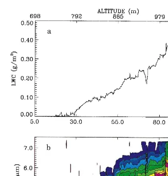
aircraft trajectory Pawlowska et al., 1997 . Fig. 1 shows an example of the variations of
Ž . Ž .
LWC in a and of the droplet spectrum in b during an ascent through the stratocumu-lus layer.
Current processing of Fast-FSSP data provides significant estimations of the droplet
Ž .
number concentration at 1 Hz 100 m spatial resolution . At higher frequencies or if droplets are sorted by size for producing a spectrum as in Fig. 1b, the number of counted particles per sample is too small for a significant estimation of their concentration, and optimal estimation is needed. Most of the droplet spectra are characterized by a mode and the relative concentration in the modal size class is much larger than the relative concentration in classes far from the modal value. It follows that the statistical significance of the concentration estimate is satisfactory at the mode but very poor on the sides. The estimation of LWC from the spectrum is thus strongly affected by the uncertainty in the estimation of the relative concentration of the biggest droplets when they are not numerous. It is, therefore, necessary to group some of the 256 Fast-FSSP size classes in order to increase the statistical significance of the measurements. The complete series of arrival times has thus been split into 16 series according to the droplet sizes. The 16 new size classes have been defined by grouping some of the 256 original classes of the instrument, in such way that the number of particles counted in each class
Ž y3 y1.
along the selected sample are similar. The relative concentration densities cm mm
in the 16 size classes have then been calculated with the optimal estimator to form a spectrum. Fig. 1b is a contour plot of the variation of that spectrum along an ascent through the cloud layer.
2
Ž . Ž .
Fig. 1. Time variation of LWC a and the droplet spectrum b along an ascent through the cloud layer with
Ž .
the M-IV. In b , the droplet spectrum is represented by the isocontours of droplet concentration density per droplet radius. The upper scale indicates the corresponding aircraft altitude.
2.2. Sampling strategy
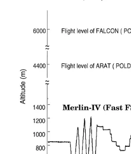
Fig. 2 shows the M-IV aircraft altitude as a function of time in mission 206. It illustrates the sampling strategy for in-situ measurements. The M-IV was flying in the cloud layer, back and forth between point M in the Southeast and point A in the Northwest, with the ARAT-F27 and the DLR-F20 flying along the same track, 2–5 km
ŽTable 1 in Brenguier and Fouquart, 2000 , above the cloud layer, for remote sensing of.
Ž .
the cloud radiative properties. The first leg from 09:30 to 09:50 UTC is at a constant
Ž .
( )
H. Pawlowska et al.rAtmospheric Research 55 2000 15–33 19
Ž . Ž
Fig. 2. Altitude vs. time for the M-IV in-situ measurements , the ARAT-F27 and the DLR-F20 for remote
. Ž
sensing , flying back and forth between points M and A that mark the end of the sampling leg Brenguier and
.
Fouquart, 2000 .
M-IV performed series of ascents and descents, extended 100 m below cloud base and 100 m above cloud top in order to document the thermodynamics outside of the cloud
Ž . Ž .
layer. The third 10:20–10:45 and fourth 10:45–11:10 legs were flown at a series of
Ž .
horizontal steps. The cloud top was slightly lower in the North A than in the South
Ž .M . During the third leg M–A , the flight level was maintained just below cloud topŽ .
and the level was lowered each time the aircraft was exiting the cloud layer. This is the reason for the descending steps in Fig. 2. On the way back to M, it was not possible to evaluate the altitude of the cloud top from inside the aircraft within the cloud layer. Therefore, the changes in flight altitude were decided on the basis of marks noted during
Ž
the previous leg the highest level during this leg is clearly lower inside the cloud than
. Ž .
the highest level during the previous one . The fifth leg 11:10–11:30 is similar to the
Ž .
second one. The last leg 11:30–11:50 is also of the zigzag type but the duration of the
Ž
ascents and descents was shortened in order to increase their number 11 profiles instead
.
Fig. 1 illustrates the limitations of the zigzag procedure. Vertical sampling is of course not feasible with an aircraft. With its rate of climbing, the M-IV is traveling about 5–10 km while it crosses the cloud thickness of about 400 m during a profile. This
Ž .
is larger than the typical scale of the cloud cells a few kilometers , as shown in the
Ž .
POLDER images Pawlowska et al., 2000 . Therefore, the variations of LWC and of the droplet spectrum in Fig. 1 do not characterize a single cell. It is clear in this example that the M-IV entered at least three cells during its ascent. Nevertheless, the cloud base altitude being about the same for all cells, their microphysical characteristics at a given level are comparable and the composite of the three cells sampled in Fig. 1 at different levels form a significant trend for LWC and the spectrum. The zigzag legs will be used in Section 3.2 to document the vertical profiles of the cloud parameters and it must be remembered that sharp changes seen in these profiles do not correspond to vertical transitions within a single cell but rather to transitions between adjacent convective cells, which are sampled successively along an aircraft ascent or descent.
3. Description of the cloud structure
3.1. General features
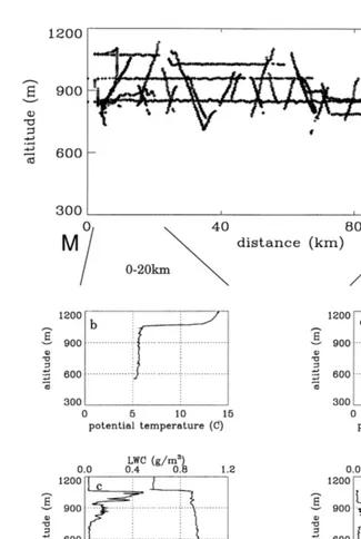
The cloud system sampled during mission 206 has two interesting features related to its spatial and temporal variations. Fig. 3a shows flight sections where LWC was detected. Each point is an average over 100 m of flight. The aircraft trajectory is reported with altitude as a function of the aircraft position along the leg M–A, with the distance measured from point M. The cloud base is located at about 750 m and slightly descending northward. The cloud top exhibits a stronger trend, descending from 1100 m at the southern edge to 900 m at the northern edge. The same features can be noted in the POLDER images with a decrease of the optical thickness from South to North
ŽPawlowska et al., 2000 . Close to point A, the layer was broken with isolated.
convective cells. Fig. 3b–d shows vertical profiles of the thermodynamics at the southern edge, with a strong and sharp inversion at the cloud top, a well-mixed boundary layer with constant potential temperature and a uniform profile of wind speed and direction. The wind direction was perpendicular to the aircraft trajectory. Fig. 3e–g shows the same parameters measured at the vicinity of point A. The inversion is broader than at the South and there is a significant wind shear through the inversion layer.
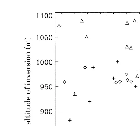
Fig. 4 summarizes both spatial and temporal variations. It represents the altitude of the base of the inversion as derived from temperature measurements for three-time
Ž . Ž .
periods covering, respectively, legs 2 and 3 10:00–10:40 , legs 4 and 5 10:40–11:30 ,
Ž .
and leg 6 11:30–12:00 . At the beginning, two regions can be identified. Up to a distance of 60 km from M, the inversion was almost reaching 1100 m, with convective cells ascending up to that level and the vertical soundings are similar to the sounding
Ž .
( )
H. Pawlowska et al.rAtmospheric Research 55 2000 15–33 21
Ž . Ž .
Fig. 3. a Trajectory of the M-IV altitude vs. distance from point M restricted to 10 m samples where LWC
Ž . Ž . Ž
is measured; b and e vertical profiles of the potential temperature within the two regions marked on a ; c
. Ž . Ž . Ž .
Fig. 4. Altitude of the base of the inversion layer estimated from temperature measurements during ascents or descents. The symbols correspond to three successive periods indicated in the upper right corner.
between M and that point is lower, at about 1000 m. During the last period, the
Ž .
inversion was broader all over the leg similar to Fig. 3e and its altitude was lower on both ends, with a maximum at almost 1000 m in the middle. This observed time evolution mainly reflects advection of large-scale structures across the sampling leg M–A. Such structures can be identified in the AVHRR satellite image at 08:25 UTC
ŽFouilloux et al., 2000 ..
3.2. VerticalÕariability
The vertical profiles of microphysics are documented with 22 M-IV ascents or descents through the cloud layer. However, as already mentioned, the sampling during an ascent or descent does not represent precisely a vertical profile in a single convective cell but rather in a series of adjacent cells. In addition, it is possible to select the top of a convective cell when starting from above cloud a descent with the aircraft, but it is difficult from inside the cloud layer to end an ascent right at the top of a convective cell. In fact, the aircraft trajectory shows that ascents and descents are regularly spaced along the legs. Despite these two limitations, impact of horizontal variability on the vertical sampling and spatial randomness of the sampling, the microphysical characteristics exhibit a remarkable trend with the vertical.
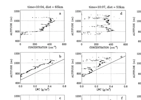
Fig. 5 presents three examples of vertical profiles of Fast-FSSP data processed with
Ž .
optimal estimation at 10 Hz Pawlowska et al., 1997 . Three parameters are displayed:
Ž .
the droplet number concentration in the 2–28 mm range a, d, g , LWC with the
Ž .
predicted adiabatic value indicated by a solid line b, e, h , and the effective radius
Žr sr3rr2. Žc, f, i , where r and r are the mean volume and mean surface radii of.
()
H.
Pawlowska
et
al.
r
Atmospheric
Research
55
2000
15
–
33
23
Ž .
the droplet size distribution, respectively. The concentration is almost constant with altitude, the lower values at the cloud base being due to the detection threshold of the Fast-FSSP at rs2,mm. Fig. 5a–c and g–i show examples of nearly adiabatic profiles of LWC, while Fig. 5d–f show evidence of dilution. As drizzle was not observed within the cloud layer, this feature can be attributed to entrainment and mixing of dry air from above the inversion. However, it can be noted that the decrease in LWC is mainly due to a decrease in number concentration while the effective radius is only slightly affected by mixing. This feature will be discussed in Section 3.3. The important point here is that the microphysics in the cloud layer is obviously varying regularly with altitude. The adiabatic model of droplet growth, with a constant droplet number concentration and LWC increasing as predicted by the solid lines in Fig. 5, represents therefore a more realistic model than a VUPPM with constant values of the microphysical parameters along the vertical.
The adiabatic model has been largely used for parameterization of the condensation
Ž
process in convective clouds Mason and Chien, 1962; Mason and Jonas, 1974; Lee and
.
Pruppacher, 1977; Brenguier, 1991 , but only occasionally for the parameterization of
Ž .
their radiative properties Boers and Mitchell, 1994 . In fact, radiative transfer calcula-tions with a VUPPM have been tested vs. vertically stratified models by considering a cloud composed of a stack of homogeneous layers whose microphysical characteristics
Ž
were specified using measured vertical profiles Slingo and Schecker, 1982; Platnick and
.
Valero, 1995 . The same procedure can be applied by deriving the microphysical properties from the adiabatic model of droplet growth. However, a stratiform cloud layer is not fully adiabatic because of mixing between the cloud and the overlying dry air or drizzle scavenging. The statistical distribution of sub-adiabaticity in the cloud layer is also an important factor to consider in a GCM parameterization scheme. This is discussed in Section 3.3.
3.3. HorizontalÕariability
The radiative properties of a cloud are mainly determined by its microphysical characteristics close to the cloud top. However, it is difficult to precisely document those characteristics, especially when the cloud top is rather inhomogeneous due to cumulus cloud turrets that overpass the mean cloud top level. In addition the cloud top is the region of highest variability in the microphysical parameters: droplet sizes are progres-sively increasing from the cloud base up to a maximum value below cloud top, above which they rapidly decrease in the narrow mixing region that separates the cloud core
Ž .
from the overlying dry air Fig. 5 . It is therefore impossible with an aircraft to locate precisely the region of maximum droplet sizes.
In EUCREX mission 206, the mean cloud top altitude was decreasing progressively from South to North and the horizontal sampling consisted of a series of horizontal
Ž
sections flown a few tens of meters below the mean cloud top see Fig. 2, legs MA:
.
( )
H. Pawlowska et al.rAtmospheric Research 55 2000 15–33 25
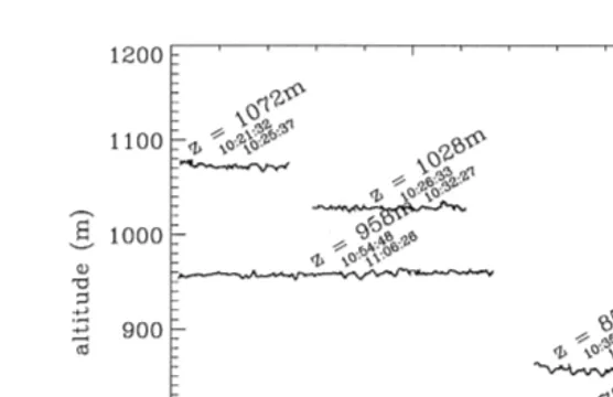
Fig. 6. Schematics of the horizontal sampling at the top of the cloud layer. For each section, the mean altitude and the start and end times of the leg are indicated.
cloud layer the plane ascended step by step at the same distance points as before, except for the last level because the cloud top height was slightly lower than during the previous leg. Two series of cloud samples are thus available at two different levels in the upper part of the cloud.
It is impossible to compare directly the results of in-situ measurements with remote sensing, because the in situ and the remote sensing aircraft were not synchronized, so there are no simultaneous measurements of the same cloud spot. In addition, the radiances measured remotely reflect integrals of the local radiative cloud properties over the whole cloud depth, while horizontal in situ sampling provides information at only one level. There is however much to learn from the horizontal statistics of the
Ž
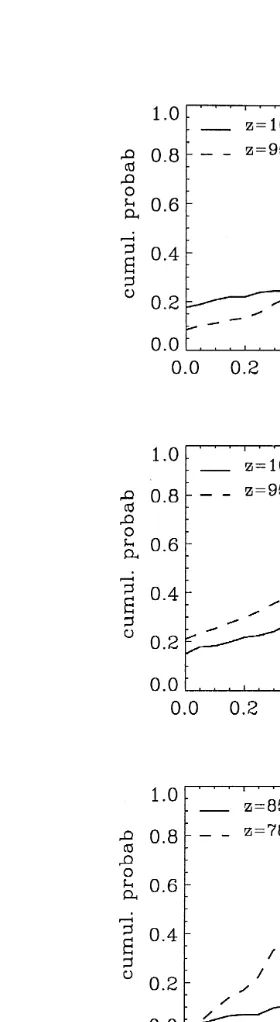
microphysical parameters. Fig. 7 summarizes the results from the first horizontal leg the
.
four highest sections in Fig. 6 at 1072, 1028, 855, and 788 m, respectively . On the left column, the data are represented in a normalized coordinate system. The x-axis corresponds to the measured concentration normalized by its adiabatic value. The
Ž .
adiabatic concentration Nad used here as a reference is calculated as the average of the maximum values measured during each cloud traverse, within the corresponding cloud section. Its value for each section is indicated in the x label between parenthesis. The
y-axis represents the mean droplet volume normalized by its adiabatic value, derived
from the formula: 4
3
rvads
ž
prwNad/
,Ž .
13
whererw is the liquid water density, and wadis the adiabatic LWC. The adiabatic LWC
Ž .
is calculated from the aircraft altitude above cloud base hszyzbase , with the cloud
Ž .
base altitude zbase estimated from Fig. 3, as indicated on top of each graph:
( )
H. Pawlowska et al.rAtmospheric Research 55 2000 15–33 27
where cw is the rate of condensation, that depends only upon pressure and temperature
Ž .
at the cloud base Brenguier, 1991 . In such a normalized system the product of the
Ž .
coordinates is proportional to wrwad where w is the measured value . The solid isolines
Ž .
represent percentages of this ratio from 10% to 100% . The data have been processed with optimal estimation at 10 Hz, that is a horizontal distance of about 10 m.
Most of the data are distributed in the area of LWC values greater than 40% of the adiabatic value. There is a significant dispersion of the measured concentrations, but the
Ž
normalized mean volume radius remains within 80% of its adiabatic value right hand
.
scale in the figure . This feature is well illustrated in the cumulative probability distributions of the normalized values of LWC, mean volume radius and number
Ž .
concentration right column in Fig. 7 . The statistics of the mean volume radius for the four sections are very similar with nearly no samples with a mean volume radius smaller than 80% of the adiabatic value. On the contrary, the droplet concentration is more uniformly distributed between 40% and 100% of the reference value. Such a feature is typical of an inhomogeneous mixing process between the cloud and the dry air from the inversion layer above. During such a process, some droplets are completely evaporated and the concentration is reduced both by dilution and loss of droplets. The remaining
Ž
droplets are then exposed to saturated air and their size is slightly affected Baker and
.
Latham, 1979 .
The distribution of wrwad evolves from a steep distribution in the southern part of the leg to a linear distribution to the North. Close to point M, the cloud layer is
Ž .
continuous and thick thickness: more than 450 m . The proportion of clear air samples is about 10% of the total and about 80% of the measured values are characterized by
w)0.6w . In the northern part of the leg, the cloud thickness is reduced to less thanad 200 m and the cloud layer is broken. The proportion of clear air samples has increased to 35% and w)0.6 wad in only 20% of the samples. It is also interesting to compare these distributions with those measured slightly lower in the cloud layer at the same place. Fig. 8 shows these distributions for both the upper and lower levels reported in Fig. 6. Except for the second section, the proportion of clear air samples is slightly reduced at the lower level. Otherwise, the distributions are quite similar indicating that the mixing, which originates from the cloud top, affects the cloud layer at a depth of more than 50 m from the cloud top.
These overall features are crucial for the parameterization of the microphysics in a GCM radiation scheme. In Section 3.2, it has been shown that a vertical stratification of the microphysics is more realistic than a vertically uniform profile, and that this stratification approaches the adiabatic model. The sampling along horizontal legs provides crucial information about the distribution of sub-adiabaticity. The distribution
Fig. 7. Left column: statistics of mean volume radius vs. droplet concentration along four of the flight sections shown in Fig. 6. Each dot corresponds to a 10-Hz sample. The droplet concentration is normalized by a reference value indicated in the x label. The mean volume radius is normalized by its adiabatic value at that
Ž 3 3 .
level rvrrvad in the left axis, rvrrvadin the right axis . Solid isolines represent the various percentages of
( )
H. Pawlowska et al.rAtmospheric Research 55 2000 15–33 29
of wrwad varies from a steep distribution in regions of homogeneous cloud deck, with most of the cloud volumes filled with almost adiabatic LWC, to a nearly linear distribution in regions of thin and broken stratocumulus. Since the in cloud light extinction is proportional to the total droplet surface, the knowledge of LWC is not sufficient for its parameterization. Information about droplet sizes is also required. The statistics of the mean volume radius as a function of droplet concentration shown in Fig. 7 suggests that a simple yet realistic hypothesis is to consider that variations of LWC with respect to the adiabatic value are due to fluctuations of the droplet concentration, while the droplet sizes remain equal to their adiabatic value at this level: NsN wad rwad
and rvsrvad.
4. Estimation of the adiabatic cloud optical thickness
An important parameter in the radiative transfer calculations in cloud is the cloud
Ž .
optical thickness which is defined as the integral of the extinction coefficient sext over
Ž .
the whole cloud depth H , i.e.
`
H H 2 H 2
ts
H
sextd hsH
QextH
pr n r d r dhŽ .
sQextpNH
r d hsŽ .
30 0 0 0
Ž .
where Qext is the mean Mie extinction factor, n r is the droplet size distribution, N is the droplet number concentration, and h is the altitude above the cloud base.
In the VUPPM approximation where the microphysical parameters are uniform along the vertical, the above equation reduces to:
3 Qext W
ts ,
Ž .
44 rw re
where WswHs4r3prwNrv3H is the LWP. Although very useful in a GCM
parame-terization, such a formula fails in describing the dependence of optical thickness as a function of cloud geometrical thickness. The cloud geometrical thickness is related to cloud dynamics and the droplet concentration reflects the level of pollution of the air mass. With the additional hypothesis of adiabaticity for the vertical profile of the
Ž .
microphysics, it is possible to explicitly calculate Eq. 3 as a function of these two parameters. In the adiabatic hypothesis, the cloud droplet concentration N is constant. Since the droplet size distributions are not monodisperse, it is necessary to express a relationship between r and r . From droplet distributions observed in stratiform clouds,v e
Ž . 3 3
Martin et al. 1994 reported values of ksrvrr , from 0.67 in continental air masses toe
Ž .
0.8 in marine ones. The adiabatic cloud optical thickness is thus derived from Eq. 3 as:
2r3
3 3cw 1r3 5r3
ts Qext
ž /
Ž
kN.
HŽ .
55 4prw
Such formula expresses that the cloud optical thickness is proportional to N1r3 as
Ž . 5r3
implicitly taken into account by replacing the droplet concentration N by a ‘‘scaled’’ droplet concentration kN. It follows that a high accuracy in k is not crucial, since the
Ž y3
aerosol indirect effect involves changes of N by a factor of up to 50 from 20 cm in
y3 .
pure marine air, to 1000 cm in polluted air .
The values of H and N measured in situ during ascents or descents will be used in
Ž . Ž .
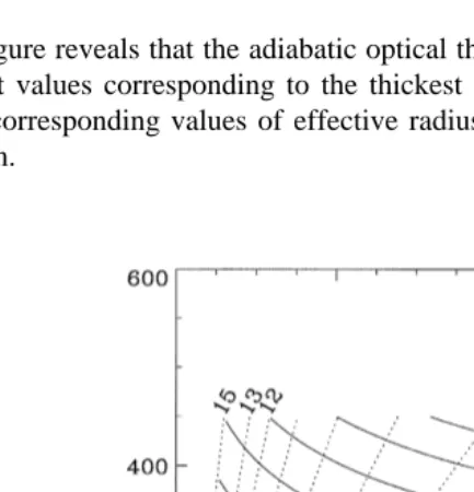
Pawlowska et al. 2000 to estimate the adiabatic optical thickness with Eq. 5 . The H and N values corresponding to the 22 cloud traverses are reported in Fig. 9. N is selected as the maximum value of concentration measured during the traverse. The
Ž .
continuous isolines represent the adiabatic cloud optical thickness derived from Eq. 5
y3 4 6 3
with Qexts2.2, cws1.5=10 grm , rws10 grm , and ks0.8. The dashed
isolines correspond to the values of the effective radius at the cloud top that can be
Ž Ž . .
derived from the above mentioned relations see also Eq. 11 in Martin et al., 1994 :
1r3
4
1r3
re
Ž
H.
srvŽ
H.
rk sž
wadŽ
H.
rž
prwkN/
/
.Ž .
63
This figure reveals that the adiabatic optical thickness varies from 8 to more than 35, the largest values corresponding to the thickest cloud layer at the southern part of the leg. The corresponding values of effective radius at the cloud top range from 6 to less than 8mm.
Fig. 9. Values of cloud geometrical thickness H and droplet concentration N for each of the 22 ascents and descents performed between points M and A. The solid isolines correspond to the adiabatic optical thickness as
Ž .
derived from Eq. 5 . The dotted isolines correspond to the effective radius at the cloud top as derived from
Ž .
( )
H. Pawlowska et al.rAtmospheric Research 55 2000 15–33 31 5. Discussion
For the numerical study of the aerosol indirect effect, parameterizations of the interaction between cloud microphysics and cloud radiative properties are needed. The primary effect of aerosol changes on cloud microphysics is to modify the droplet concentration. Therefore, empirical parameterizations are not suited if they cannot capture the basis of the relationship between the droplet concentration and cloud radiative properties. At the scale of a cloud system, the large variability of the droplet concentration that results from variability of the cloud nuclei activation process, from mixing processes between the cloud and the overlying dry air, and from drizzle scavenging prevents the observation of such relationships. However, within a convective core, the droplet concentration is almost constant and the vertical evolution of the microphysics follows simple laws.
The objectives in EUCREX were to document precisely this vertical evolution in order to support the use of the adiabatic microphysical model for parameterization of the optical thickness at the scale of a cloud cell. The second step is to document the horizontal variability of the cloud microphysics with respect to the adiabatic reference. The vertical evolution has been observed via series of short ascents and descents through the cloud layer. They confirm previous observations in similar clouds, namely that LWC is close to its adiabatic value, that the droplet concentration is almost constant and that the droplet sizes are increasing according to the adiabatic model. The model has
Ž .
then been used to estimate the maximum values i.e., adiabatic of optical thickness at different locations within the cloud system. These estimates are compared in the conclusion paper of values derived from radiometric measurements from above the cloud layer.
The effects of the mixing and of the resulting variability of the microphysical field on the radiation field are more difficult to characterize and parameterize. We believe that cloud-resolving simulations of 3D cloud fields will be necessary, with detailed radiative transfer calculations. Such models can be used to simulate various levels of variability and, after integration over the whole domain of simulation, to establish parameteriza-tions between the mean dynamical properties of a cloud system and its mean radiative properties. However, most of the cloud resolving models are predicting only LWC and even models with detailed microphysics cannot simulate explicitly the effects of mixing on droplets because this process proceeds at very small scales, down to a few centimeters, that is scales smaller than the model grid. For validation of the numerical simulations, it is thus crucial to document the statistics of the microphysics, including the effects of mixing processes on droplet sizes.
Series of horizontal legs have been performed close to cloud top to document this second aspect of the problem. They reveal that the variability in LWC is more important in thin cloud layers than in thicker clouds where a large percentage of the values remain within 60–100% of the adiabatic value. In addition, it appears that the variability in LWC is mainly due to a variability in the droplet concentration while the droplet sizes remain close to their adiabatic values at the corresponding level. Such a feature can be simply implemented in a cloud-resolving model. Once w is known in a grid box, the
Ž .
Ž . 1r3
resrvad hrk . The results of the statistical analysis on the distributions of LWC, N and rv are summarized in a series of cumulative distributions over horizontal cloud sections sampled during the EUCREX mission 206.
Ž
The cloud system described in this study is typical of a polluted air mass Nf400
y3.
cm . In particular, there was no production of drizzle in the EUCREX mission 206 cloud system, while drizzle scavenging is also likely to play an important role in the
Ž
spatial variability of the microphysics and the life time of the cloud system Vali et al.,
.
1998 . Additional measurements of the same type are thus necessary in pure marine and slightly polluted air masses in order to demonstrate the indirect effect of aerosols on climate and provide complementary observations for validation of the numerical models.
Ž .
The ACE-2 Aerosol Characterization Experiment is a good opportunity for such measurements.
Acknowledgements
The authors are grateful to the Meteo-France Merlin-IV teams for their efficient contribution to the data collection and to the GMEIrMMA for data processing. This work has been supported by INSU-PATOM under grant 94r08 and by the European Union Environment and Climate Division, under grant ENV4-CT95-0117.
References
Baker, M.B., Latham, J., 1979. The evolution of droplet spectra and rate of production of embryonic raindrops in small cumulus clouds. J. Atmos. Sci. 36, 1612–1615.
Barker, H.W., 1992. Solar radiative transfer through clouds possessing isotropic variable extinction coefficient. Q. J. R. Meteorol. Soc. 118, 1145–1162.
Barker, H.W., 1996. Estimating cloud field albedo using one-dimensional series of optical depth. J. Atmos. Sci. 53, 2826–2837.
Boers, R., Mitchell, R.M., 1994. Absorption feedback in stratocumulus clouds: influence on cloud top albedo. Tellus A 46, 229–241.
Brenguier, J.L., 1991. Parameterization of the condensation process: a theoretical approach. J. Atmos. Sci. 48, 264–282.
Brenguier, J.L., Fouquart, Y., 2000. Introduction to the EUCREX-94 mission 206. Atmos. Res., This issue. Brenguier, J.L., Bourrianne, T., Coelho, A.A., Isbert, J., Peytavi, R., Trevarin, D., Wechsler, P., 1998. Improvements of the droplet size distribution measurements with the Fast-FSSP. J. Atmos. Oceanic Technol. 15, 1077–1090.
Coley, P.F., Jonas, P.R., 1997. The contribution of cloud inhomogeneities and droplet concentration to the albedo of broken-cloud fields. Q. J. R. Meteorol. Soc. 123, 1931–1944.
Coakley, J.A. Jr., Chylek, P., 1975. The two-stream approximation in radiative transfer: including the angle of´ the incident radiation. J. Atmos. Sci. 32, 409–418.
Davis, A., Marshak, A., Wiscombe, J.W., Cahalan, R., 1996. Scale invariance of liquid water distributions in marine stratocumulus: Part I. Spectral properties and stationarity issues. J. Atmos. Sci. 53, 1538–1558. Duda, D.P., Stephens, G.L., Stevens, B., Cotton, W.R., 1996. Effects of aerosols and horizontal inhomogeneity
on the broadband albedo of marine stratus: numerical simulations. J. Atmos. Sci. 53, 3757–3769. Fouilloux, A., Gayet, J.F., Kriebe, K.T., 2000. Determination of cloud microphysical properties from AVHRR
images: comparisons of three approaches. Atmos. Res., This issue.
( )
H. Pawlowska et al.rAtmospheric Research 55 2000 15–33 33 Hignett, P., Taylor, J.P., 1996. The radiative properties of inhomogeneous boundary layer cloud: observations
and modelling. Q. J. R. Meteorol. Soc. 122, 1341–1364.
Lee, I.Y., Pruppacher, H.R., 1977. A comparative study of the growth of cloud droplets by condensation using an air parcel model with and without entrainment. Pure Appl. Geophys. 115, 523–545.
Li, J., Geldart, J.W., Chylek, P., 1994. Solar radiative transfer in clouds with vertical internal inhomogeneity.´ J. Atmos. Sci. 51, 2542–2552.
Martin, G.M., Johnson, D.W., Spice, A., 1994. The measurement and parameterization of effective radius of droplets in warm stratocumulus clouds. J. Atmos. Sci. 51, 1823–1842.
Mason, B.J., Chien, C.W., 1962. Cloud droplet growth by condensation in cumulus. Q. J. R. Meteorol. Soc. 88, 136–142.
Mason, B.J., Jonas, P.R., 1974. The evolution of droplet spectra and large droplets by condensation in cumulus clouds. Q. J. R. Meteorol. Soc. 100, 23–38.
Nicholls, S., 1984. The dynamics of stratocumulus: aircraft observations and comparisons with a mixed layer model. Q. J. R. Meteorol. Soc. 110, 783–820.
Pawlowska, H., Brenguier, J.L., Salut, G., 1997. Optimal nonlinear estimation for cloud particle measure-ments. J. Atmos. Oceanic Technol. 14, 88–104.
Pawlowska, H., Brenguier, J.L., Fouquart, Y., Armbruster, W., Bakan, S., Descloitres, J., Fischer, J., Flamant, C., Fouilloux, A., Gayet, F., Ghosh, S., Jonas, P., Parol, F., Pelon, J., Schuller, L., 2000. Microphysical¨ and radiative properties of stratocumulus cloud: the EUCREX mission 206 case study. Atmos. Res., This issue.
Platnick, S., Valero, F.P.J., 1995. A validation of satellite cloud retrieval during ASTEX. J. Atmos. Sci. 52, 2985–3001.
Slingo, A., 1989. A GCM parameterization for the shortwave radiative properties of water clouds. J. Atmos. Sci. 46, 1419–1427.
Slingo, A., Schrecker, H.M., 1982. On the shortwave radiative properties of stratiform water clouds. Q. J. R. Meteorol. Soc. 108, 407–426.
Slingo, A., Nicholls, S., Schmetz, J., 1982. Aircraft observations of marine stratocumulus during JASIN. Q. J. R. Meteorol. Soc. 108, 833–856.
Stephens, G.L., 1978. Radiation profiles in extended water clouds: II. Parameterization schemes. J. Atmos. Sci. 35, 2123–2132.
Stephens, G.L., Platt, C.M.R., 1987. Aircraft observations of the radiative and microphysical properties of stratocumulus and cumulus cloud fields. J. Clim. Appl. Meteorol. 26, 1243–1269.
Twomey, S., 1977. The influence of pollution on the shortwave albedo of clouds. J. Atmos. Sci. 34, 1149–1152.
Twomey, S., Jacobowitz, H., Howell, H.B., 1966. Matrix methods for multiple scattering problems. J. Atmos. Sci. 23, 101–108.