______________________________
CALIBRATION OF MULTI-CAMERA PHOTOGRAMMETRIC SYSTEMS
I. Detchev a, M. Mazaheri a, *, S. Rondeel a, A. Habib b a
Department of Geomatics Engineering, University of Calgary, 2500 University Drive NW, Calgary, Alberta, Canada T2N 1N4 – (i.detchev, m.mazaheri, sjrondee)@ucalgary.ca
b
Lyles School of Civil Engineering, Purdue University, 550 Stadium Mall Drive, West Lafayette, Indiana, USA 47907-2051 – [email protected]
Commission I, WG I/3
KEY WORDS: digital close range photogrammetry, geometric camera calibration, bundle adjustment, multisensor systems
ABSTRACT:
Due to the low-cost and off-the-shelf availability of consumer grade cameras, multi-camera photogrammetric systems have become a popular means for 3D reconstruction. These systems can be used in a variety of applications such as infrastructure monitoring, cultural heritage documentation, biomedicine, mobile mapping, as-built architectural surveys, etc. In order to ensure that the required precision is met, a system calibration must be performed prior to the data collection campaign. This system calibration should be performed as efficiently as possible, because it may need to be completed many times. Multi-camera system calibration involves the estimation of the interior orientation parameters of each involved camera and the estimation of the relative orientation parameters among the cameras. This paper first reviews a method for multi-camera system calibration with built-in relative orientation constraints. A system stability analysis algorithm is then presented which can be used to assess different system calibration outcomes. The paper explores the required calibration configuration for a specific system in two situations: major calibration (when both the interior orientation parameters and relative orientation parameters are estimated), and minor calibration (when the interior orientation parameters are known a-priori and only the relative orientation parameters are estimated). In both situations, system calibration results are compared using the system stability analysis methodology.
1. INTRODUCTION
Photogrammetric systems for three-dimensional (3D) reconstruction often include multiple cameras which are rigidly mounted to a frame. Having a correct and strong system calibration is essential for accurate object point determination. This is especially crucial for a number of scenarios such as: direct sensor orientation in mobile mapping applications (Ellum and El-Sheimy, 2002; Rau et al., 2011), dense image matching for full surface/object reconstruction (Remondino and El-Hakim, 2006; Remondino et al., 2008), infrastructure monitoring (Detchev et al., 2013; Kwak et al., 2013), biomedical and motion-capture metric applications (D’Apuzzo, 2002; Detchev et al., 2011; Remondino, 2004), and the generation of photo scenes from multiple sensors (Tommaselli et al., 2013).
For a photogrammetric system, the interior orientation parameters (IOPs) for the involved cameras should ideally be estimated prior to any data collection campaign. However, in the case when a system consists of many cameras and/or disassembling them from the platform is not desirable, the IOP estimation must be done in-situ or on-the-job. The challenge of such an IOP calibration approach is to guarantee adequate network geometry, e.g., multi-station convergent images with a good base-to-depth ratio and sufficient tie points which are distributed evenly within the image format of each camera. This network configuration can be simulated by translating and rotating a portable test field, while keeping the camera system in place.
This paper first reviews a method for multi-camera system calibration. This calibration can handle both the estimation of
the IOPs for each individual camera and the estimation of the relative orientation parameters (ROPs) of each camera with respect to a body frame or a reference camera. IOPs define the interior geometry of individual cameras in an attempt to reconstruct the bundle of light rays at the moment of exposure. ROPs are also known as the mounting parameters of the cameras to the system platform and define the position and attitude of the cameras relative to one another.
The objective of the paper is to find out the most optimal calibration configurations for a photogrammetric system used for a long-term biomedical application. There are two scenarios for the system calibration: major calibration, when both the IOPs and the ROPs of the involved cameras are determined simultaneously; and minor calibration, when the IOPs are assumed to be known, and only the ROPs are estimated. The paper shows the results from a full calibration data set, which includes multiple redundant sets of images, and the results from several data sets, whose number of redundant sets of images have been progressively reduced. A method for system stability analysis is described, which can be used as a tool to compare the different sets of system calibration parameters. The system stability analysis method investigates whether or not there are significant changes in the estimated IOPs or ROPs coming from the full calibration data set versus the several sub-sampled calibration data sets.
2. MATHEMATICAL MODELS FOR CALIBRATION OF MULTI-CAMERA SYSTEMS
In general, the calibration parameters for a multi-camera photogrammetric system include the IOPs and ROPs. The IOPs include the principal point offset ( , ), the principal distance
( ), and any additional parameters describing distortions in the image space (e.g., , , , , ). Assuming that the ROPs are defined to be relative to a reference camera, they consist of the lever arm/spatial ( ) and the boresight/rotational ( offsets between the individual cameras ( ) and the reference one ( ). There exist two-step and one-step procedures for estimating the ROPs. The following mathematical models are based on the assumption that the camera IOPs and ROPs are block invariant, i.e., they remain stable from one observation epoch to the next within a given data collection campaign. The two-step procedure first estimates the exterior orientation parameters (EOPs) for the different cameras through a conventional bundle block adjustment based on the collinearity equations (1). The ROPs are then derived from the EOPs using equations (2) and (3). As a final result, the time-dependant ROPs can be averaged, and their standard deviations can be computed.
( ( ( (1)
( ( ( ( ( ( (2)
( ( ( ( (3)
The one-step procedure is usually based on constrained equations, which enforce an invariant geometrical relationship between the cameras at different observation epochs. For example, if the number of cameras involved in the system is , and the number of observation epochs is , then the total number of EOPs is . Assuming that the lever arm and boresight components are not changing over time, the number of constraints that can be introduced is ( ( . Thus, the number of independent parameters that define the EOPs of the different cameras at all the observation epochs is
( . The downside of using such relative orientation constraints is that the complexity of the implementation procedure intensifies with the increase of the number of cameras in the system and the number of observation epochs.
In this paper, a single-step procedure is utilized which directly incorporates the relative orientation constraints among all cameras and the body frame/reference camera in the collinearity equations (4) (Habib et al., 2014; Rau et al., 2011).
( ( ( ( (4)
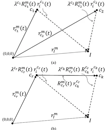
The ROPs, and , are now time-independent, and the EOPs of the reference camera, ( and ( , now represent the EOPs of the system platform. This model preserves its simplicity regardless of the number of cameras or the number of observation epochs. It should be noted that instead of solving for EOP unknowns, the adjustment will solve for EOPs for the reference camera in addition to ( ROPs for the rest of the cameras with respect to the reference camera. This is equivalent to the total number of independent parameters that are needed to represent the EOPs of the different cameras at all the data acquisition epochs. The reduction in the number of parameters in the adjustment will also reduce any possible high correlations between the many system calibration parameters. The difference in the bundle adjustment mathematical models described in equations (1) and (4) is visually summarized in Figure 1.
(a)
(b)
Figure 1. Mathematical model for multi-camera calibration using separate EOPs for each camera station (a) versus using EOPs for a reference camera and ROPs for the rest of the cameras (b) (Habib et al., 2014) There are situations when both the IOPs and the ROPs of a multi-camera system must be estimated. For example, if the system is assembled for the first time, re-assembled after transportation or used in a location, where the atmospheric conditions frequently change, such a major calibration will be required. However, if the IOPs are believed not to change significantly over a certain period of time, and only the ROPs must be fine-tuned due to handling of the system frame, a minor calibration would suffice. Again, a minor calibration includes the estimation of only the ROPs. This paper will investigate different configurations for both the major and minor calibration configurations. The results from these different configurations will be compared using a methodology for multi-camera system stability analysis, which is described next.
3. METHODOLOGY FOR SYSTEM STABILITY ANALYSIS
The objective of a system stability analysis procedure is to decide whether the cumulative effect on the 3D reconstruction process for two sets of IOPs and ROPs is equivalent or not. In other words, for a given image data set, do the 3D reconstruction results differ depending on the set of system calibration parameters used?
Here a methodology will be presented that simultaneously compares two IOP sets, ( and ( with ( and ( , and two ROP sets, ( and ( with
( and ( , for two camera stations, and , derived from two calibration sessions or two different calibration configurations, and . Since the ROPs output from a system calibration at a specific time, , are actually ( , ( ,
( and ( , the desired ROPs for comparison are computed using equations (5) and (6):
( ( ( ( ( ( (5)
( ( ( ( (6)
The methodology for system stability analysis is simulation-based, i.e., a synthetic grid in image space is used for evaluating the stability of the system parameters; the actual system parameters to be tested are real, not simulated. The method is briefly explained here:
Define a synthetic regular grid in the image space of one of the cameras, ;
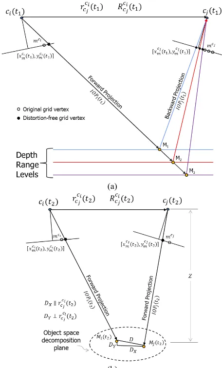
Use the IOPs and ROPs of this camera from the first calibration session or configuration to remove the distortions at the grid vertices and compute the object space coordinates of each vertex by forward projecting them to a range of plausible object space depths (see Figure 2a);
Compute the image space coordinates of the grid points for the other camera, , by backward projection using the IOPs and ROPs for the other camera from the first calibration session or configuration (see Figure 2a). Note that different depth values will each yield unique “grids” in the image space of the second camera;
Estimate the effect of the IOPs and ROPs obtained from another calibration session or configuration, in image units (i.e., pixels), for all simulated points and depth levels by computing the object space parallax (see Figure 2b). The object space parallax or discrepancy arising from the variations in the IOPs and ROPs for both cameras is evaluated by forward projecting the grid vertices within an object space plane (see Figure 2b). This object space parallax or discrepancy is decomposed into - and -components, and , where is parallel, and is perpendicular to the baseline between the two cameras (see Figure 2b). These two components are then converted to image space units by scaling them with the ratio between the average principal distance,
( , and the object space depth, ;
Compare the root mean squared error (RMSE) value for all the differences/offsets to the expected or required image space coordinate measurement precision; if the RMSE value is the smaller one, then the system is deemed stable or the two calibration configurations are considered compatible, and if the RMSE value is the greater one, the system would be deemed unstable or the two calibration configurations would not be considered compatible.
For more details on this method for system stability analysis one can refer to Habib et al. (2014).
4. EXPERIMENTAL RESULTS AND DISCUSSION
A multi-camera photogrammetric system was set up to be used for a biomedical application related to monitoring the progression of scoliosis via modelling the human torso in 3D (see Figure 3). The system was comprised of seven digital single-lens reflex (DSLR) cameras, namely Canon EOS 1100D/Rebel T3. This model had a 22.2 x 14.7 mm2 complementary metal-oxide semiconductor (CMOS) sensor divided into 4272 x 2848 pixels or 12.2 mega pixels, with each pixel being approximately 5.2 x 5.2 µm2. The focal lengths of the lenses were set to the nominal value of 30 mm.
(a)
(b)
Figure 2. Forward and backward projections with the first set of system calibration parameters (a); forward projections with the second set of system calibration parameters for quantifying the object space parallax (b) (Habib et al., 2014)
Figure 3. Multi-camera photogrammetric system consisting of seven DSLRs attached to a metal frame
In order for the aspect ratio of the image format to be proportional to the dimensions of the object of interest (i.e., the human body) the system was designed with each camera oriented in portrait mode (i.e., the -axis of its coordinate system being in the vertical direction) (see Figure 3 and Figure 4a). The test field used for the system calibration was a relatively flat, i.e., two-dimensional (2D), board with a seven by nine grid of checkerboard targets and a four by three grid of coded targets. The origin of the local coordinate system was at
the central checkerboard target, the orientations of the , and axes were chosen in such a way as to avoid the gimbal lock, and the coded targets were used for automating the target labelling/correspondence problem (see Figure 4b).
(a) (b)
Figure 4. The coordinate system used for a particular camera (a); the calibration test field showing the origin and the orientation of the local coordinate system (b) The system is being used almost daily for 4-5 hours at a time by non-photogrammetrists. This type of frequent use of the system leads to unknown and unpredictable changes, and thus frequent calibrations help ensure that accurate results can always be obtained. The authors chose to calibrate the system IOPs and ROPs simultaneously, i.e., to perform a major calibration, on a weekly basis, and to calibrate the ROPs only, i.e., to perform a minor calibration, on a daily basis. The next two sub-sections will attempt to find out the most optimal calibration configurations for the major and minor calibration cases. 4.1 Major calibration configurations
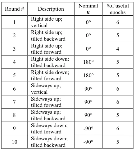
In order to avoid projective compensation or correlation between the interior and exterior orientation parameters, convergent geometry and a roll of the test field was implemented by taking images in multiple rounds consisting of multiple epochs. Each round was represented by a certain position and orientation of the test field with respect to the reference camera. Examples of different orientations would be quad rolling or placing the test field at a angle of 0° (right side up), 180° (right side down) or ±90° (sideways up or down) around the axis, and keeping it vertical, tilted forward or tilted backward. Note that the 0° and 180° orientations of the test field were in the object space portrait mode, thus matching the aspect ratios of the camera orientations. The test field was sequentially rotated at equal increments for each of the listed orientations. Each increment of the test field represented a separate epoch. Generally, six epochs were executed per round, from which at least four were useful for the bundle adjustment. A useful epoch means that the test field was within the field of view of the reference camera. If the test field was not visible by the reference camera at a particular epoch, that epoch was discarded from the adjustment. Also, four to seven cameras photographed useful images of the test field per epoch. Altogether, there were two to six images per camera per round that could be used in the calibration adjustment. In total, ten rounds were completed for a full major calibration. For a written description of the target field orientation and the number of useful epochs for each of the data collection rounds see Table 1.
Round # Description Nominal #of useful epochs 1 Right side up;
vertical 0° 6
2 Right side up;
tilted backward 0° 5
3 Right side up;
tilted forward 0° 4
4 Right side down;
tilted backward 180° 5
5 Right side down;
tilted forward 180° 5
6 Sideways up;
vertical 90° 6
7 Sideways up;
tilted forward 90° 6
8 Sideways up;
tilted backward 90° 5
9 Sideways down;
tilted forward -90° 6
10 Sideways down;
tilted backward -90° 5
Table 1. Description of the target field orientation for the ten rounds of data collection
It should be mentioned here that the camera system is designed to capture images in all cameras simultaneously regardless of whether the test field falls within the field of view of all the cameras or not. This leads to an extremely high volume of acquired images, many of which are unusable in the calibration. A semi-automatic clean-up of the raw data is performed to eliminate the images, in which the test field is either not clearly visible or it is too oblique. However, even after this clean-up of the raw data, the number of observed images and targets per camera far exceeded what is normally required for an acceptable single camera calibration. Also, collecting ten rounds was considered too time consuming. Due to these reasons, the full ten-round major calibration data set was sub-sampled in three different ways:
Rounds 1, 2, 3, 4, 5 and 6 – medium sub-sampling as to maximize the number of visible targets per image by matching the aspect ratio of the test field with the orientation the cameras for the majority of the rounds; Rounds 1, 2, 3, 6, 7 and 8 – medium sub-sampling as
to preserve the geometrical balance between the portrait and landscape orientations of the test field; Rounds 1, 2, 3 and 6 – minimum sub-sampling as to
include forward and backward tilts and at least one rolled round.
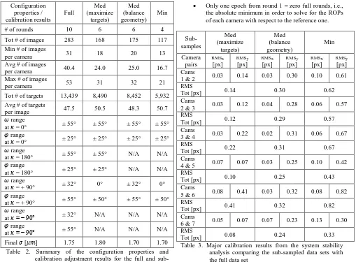
This was done in order to decide how many rounds would be sufficient for a more realistic major calibration data collection campaigns in the future. Table 2 summarizes the number of rounds, images and targets used; the ranges of and at the specific orientations for the reference camera; and the final value for each particular calibration adjustment.
Since the full ten-round calibration had the greatest redundancy and the most well-rounded network geometry, it was taken as the reference with which to compare the system calibration results from the other three sub-sampled data sets. Table 3 summarizes the root mean squared (RMS) values between the full and the sub-sampled calibrations.
Configuration
All three sub-sampled calibrations achieved results comparable with the full calibration in the case the required image space precision was one pixel. However, if the expected image space precision of 1.8 or approximately 1/3 of a pixel was to be strictly considered, the medium six-round calibration, which has the most balanced network geometry, would be the preferred configuration to use in future major calibration data collection campaigns.
4.2 Minor calibration configurations
Again, in a minor calibration only the ROPs are solved for. The experimental configurations for the tested minor calibrations were even smaller sub-samples of the full calibration data set. Minor calibrations need to be collected quickly and possibly multiple times per day by non-photogrammetrists. This led to the decision that the possible minor calibration configurations should be three rounds or less. Note that since estimating the IOPs is not part of a minor calibration, a round where the test field is rolled at ±90° was not required. Here is a list of the chosen sub-sampled configurations for the minor calibration:
Rounds 1, 2, and 4 – three full rounds or the maximum number of practically allowed rounds, where there is both lots of redundancy and good network geometry;
Rounds 2 and 4 – two full rounds with sufficient redundancy and relatively strong network geometry; Round 1 – one full round to have some redundancy
for the ROP estimation;
Only one epoch from round 1 – zero full rounds, i.e., the absolute minimum in order to solve for the ROPs of each camera with respect to the reference one.
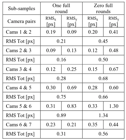
Sub-analysis comparing the sub-sampled data sets with the full data set sampled minor calibrations. The differences in the actual estimated ROPs can be seen in Tables 7-14 listed in the Appendix.
Strictly speaking none of the minor calibrations had all their camera pairs meet the expected precision of 1/3 of a pixel. However, the required precision for this particular application is one pixel, so the only minor calibration, which did not meet this requirement, was the one with the bare minimum number of images, marked as zero full rounds. Finally, it was decided that the configuration with two full rounds would be used for future minor calibration data collection campaigns. The decision was based on the trade-off between saving time, and having sufficient redundancy and a relatively strong network geometry. 5. CONCLUSIONS AND RECOMMENDATIONS FOR
FUTURE WORK
This paper first reviewed a method for a single-step calibration of multi-camera photogrammetric systems. The objective of the paper was to find out the optimal number of image rounds that need to be collected in order to perform either a major or a minor system calibration. The idea was to minimize the time it took for the data acquisition process, while preserving the necessary precision for the estimated system parameters. The
paper also reviewed a method for system stability analysis, which was used to compare the calibration parameter sets from different system configurations. Several calibrations of a seven-camera photogrammetric system used for a biomedical application were performed. Due to its frequent use, the system requires a complete IOP and ROP calibration, i.e., a major calibration, once a week, and an ROP only calibration, i.e., a minor calibration, every day. By using the system stability analysis method as a tool for comparing the different major and minor calibrations, it was possible to identify the most practical configurations for both the major and minor calibration situations. calibration adjustment results for the sub-sampled minor calibrations analysis comparing the three and two full round sub-sampled minor calibration data sets with the full analysis comparing the one and zero full round sub-sampled minor calibration data sets with the full major calibration data set
Future work will include more testing of the listed methods on different multi-camera systems. In particular, the calibration of a photogrammetric system, whose cameras exhibit near-normal network geometry and whose image footprints do not overlap 100%, will be investigated. Moreover, a method for including all observed epochs, regardless of whether the test field is visible by the reference camera or not, will be implemented.
ACKNOWLEDGEMENTS
The authors would like to thank TECTERRA for funding this research project. Also, the help of the following individuals is much appreciated: Fangning He and Zahra Lari from the Digital Photogrammetry Research Group (DPRG), and Jessica Küpper, Alexandra Melia and Sarah Sanni from Dr. Janet Ronsky’s research team.
LIST OF REFERENCES
D’Apuzzo, N., 2002. Surface measurement and tracking of human body parts from multi-image video sequences. ISPRS Journal of Photogrammetry and Remote Sensing 56, 360–375. doi:10.1016/S0924-2716(02)00069-2 deformation measurements with off-the-shelf digital cameras. Journal of Applied Geodesy 7, 147–157. doi:10.1515/jag-2012-0052
Ellum, C., El-Sheimy, N., 2002. Land-based mobile mapping systems. Photogrammetric Engineering & Remote Sensing 68, 13–28.
Habib, A., Detchev, I., Kwak, E., 2014. Stability Analysis for a Multi-Camera Photogrammetric System. Sensors 14, 15084–15112. doi:10.3390/s140815084
Kwak, E., Detchev, I., Habib, A., El-Badry, M., Hughes, C., 2013. Precise Photogrammetric Reconstruction Using
Model-Based Image Fitting for 3D Beam Deformation Monitoring. Journal of Surveying
Engineering 139, 143–155.
doi:10.1061/(ASCE)SU.1943-5428.0000105
Rau, J.-Y., Habib, A.F., Kersting, A.P., Chiang, K.-W., Bang, K.-I., Tseng, Y.-H., Li, Y.-H., 2011. Direct Sensor Orientation of a Land-Based Mobile Mapping
System. Sensors 11, 7243–7261.
doi:10.3390/s110707243
Remondino, F., 2004. 3-D reconstruction of static human body shape from image sequence. Computer Vision and
Image Understanding 93, 65–85.
doi:10.1016/j.cviu.2003.08.006
Remondino, F., El-Hakim, S., 2006. Image-based 3D Modelling: A Review. The Photogrammetric Record 21, 269–291. doi:10.1111/j.1477-9730.2006.00383.x Remondino, F., El-Hakim, S.F., Gruen, A., Zhang, L., 2008.
Turning images into 3-D models. IEEE Signal Processing Magazine 25, 55 –65. doi:10.1109/MSP.2008.923093
Tommaselli, A.M.G., Galo, M., de Moraes, M.V.A., Marcato, J., Caldeira, C.R.T., Lopes, R.F., 2013. Generating Virtual Images from Oblique Frames. Remote Sensing 5, 1875–1893. doi:10.3390/rs5041875
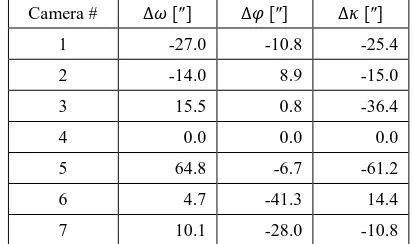
APPENDIX
The Appendix contains the differences in the spatial and rotational components of the ROPs between the sub-sampled minor calibrations and the full major calibration.
Camera # [m] [m] [m]
1 0.0001 0.0001 -0.0002
2 0.0000 0.0000 0.0000
3 0.0000 -0.0002 0.0001
4 0.0000 0.0000 0.0000
5 -0.0001 -0.0006 -0.0002
6 -0.0003 0.0000 0.0000
7 -0.0002 0.0000 -0.0001
Table 7. Differences in the spatial components of the ROPs between the three-round minor calibration and the full major calibration
Camera # [″] [″] [″]
1 -37.1 16.5 -4.8
2 4.7 -2.2 -13.0
3 40.0 3.0 -29.0
4 0.0 0.0 0.0
5 89.6 -17.6 -39.6
6 -2.5 -42.5 21.6
7 14.8 -24.3 21.6
Table 8. Differences in the rotational components of the ROPs between the three-round minor calibration and the full major calibration
Camera # [m] [m] [m]
1 0.0001 0.0001 -0.0002
2 0.0000 -0.0001 0.0001
3 0.0000 -0.0004 0.0001
4 0.0000 0.0000 0.0000
5 -0.0001 -0.0005 -0.0002
6 -0.0003 0.0000 0.0000
7 -0.0001 0.0000 0.0000
Table 9. Differences in the spatial components of the ROPs between the two-round minor calibration and the full major calibration
Camera # [″] [″] [″]
1 -38.5 24.0 9.6
2 24.8 -5.0 -12.7
3 54.7 3.7 -24.2
4 0.0 0.0 0.0
5 76.3 -16.6 -21.6
6 -1.1 -41.4 14.4
7 1.4 -13.9 28.8
Table 10. Differences in the rotational components of the ROPs between the two-round minor calibration and the full major calibration
Camera # [m] [m] [m]
1 -0.0001 0.0000 -0.0001
2 0.0000 0.0000 0.0000
3 0.0000 -0.0001 0.0001
4 0.0000 0.0000 0.0000
5 -0.0001 -0.0004 -0.0002
6 -0.0003 0.0000 0.0000
7 -0.0002 0.0000 -0.0001
Table 11. Differences in the spatial components of the ROPs between the one-round mini calibration and the full major calibration
Camera # [″] [″] [″]
1 -27.0 -10.8 -25.4
2 -14.0 8.9 -15.0
3 15.5 0.8 -36.4
4 0.0 0.0 0.0
5 64.8 -6.7 -61.2
6 4.7 -41.3 14.4
7 10.1 -28.0 -10.8
Table 12. Differences in the rotational components of the ROPs between the one-round minor calibration and the full major calibration
Camera # [m] [m] [m]
1 0.0001 -0.0002 0.0000
2 0.0003 -0.0003 0.0002
3 0.0001 -0.0003 0.0003
4 0.0000 0.0000 0.0000
5 0.0002 -0.0003 -0.0001
6 -0.0001 0.0004 0.0002
7 0.0000 0.0003 0.0001
Table 13. Differences in the spatial components of the ROPs between the single-epoch minor calibration and the full major calibration
Camera # [″] [″] [″]
1 -37.8 19.2 6.8
2 9.4 48.9 4.6
3 38.2 19.9 -20.8
4 0.0 0.0 0.0
5 60.8 40.1 -82.8
6 -33.8 -11.8 -25.2
7 2.5 -1.5 -36.0
Table 14. Differences in the rotational components of the ROPs between the single-epoch minor calibration and the full major calibration