MULTI-TEMPORAL LAND COVER CLASSIFICATION WITH LONG SHORT-TERM
MEMORY NEURAL NETWORKS
M. Rußwurm∗
, M. K¨orner
Technical University of Munich, Chair of Remote Sensing Technology, Computer Vision Research Group Arcisstraße 21, 80333 Munich, Germany –{marc.russwurm,marco.koerner}@tum.de
Commission III, WG III/7
KEY WORDS:Long Short-Term Memory, Recurrent Neural Networks, Sentinel 2, Crop Identification, Deep Learning, Land Cover Classification
ABSTRACT:
Land cover classification (LCC)is a central and wide field of research in earth observation and has already put forth a variety of classification techniques. Many approaches are based on classification techniques considering observation at certain points in time. However, some land cover classes, such as crops, change their spectral characteristics due to environmental influences and can thus not be monitored effectively with classical mono-temporal approaches. Nevertheless, these temporal observations should be utilized to benefit the classification process. After extensive research has been conducted on modeling temporal dynamics by spectro-temporal profiles using vegetation indices, we propose a deep learning approach to utilize these temporal characteristics for classification tasks. In this work, we show howlong short-term memory(LSTM) neural networks can be employed for crop identification purposes with SENTINEL 2A observations from large study areas and label information provided by local authorities. We compare these temporal neural network models,i.e., LSTMandrecurrent neural network(RNN), with a classical non-temporalconvolutional neural network(CNN) model and an additionalsupport vector machine(SVM) baseline. With our rather straightforward LSTM variant, we exceeded state-of-the-art classification performance, thus opening promising potential for further research.
1. INTRODUCTION
In earth observation, the problem domain ofland cover classifica-tion(LCC) has educed a variety of techniques until today. Many approaches rely on mono-temporal observations and concentrate onspectralortexturalfeatures describing observations acquired at one specific point in time. However, some land cover classes— such as,e.g., vegetation and especially crops—are difficult to classify by mono-temporal approaches (Foerster et al., 2012), as vegetation changes its spectral and textural appearance within its species-dependent growth cycle. Especially crops develop these temporal dynamics in a systematic and thus predictable manner, dependent on phenology and the applied crop calendar (Valero et al., 2016; Whitcraft et al., 2014). Thesetemporalfeatures can be utilized for classification by suitable techniques.
In the recent past, thedeep learningcommunity has developed a variety of architectures producing impressive results for a wide range of applications. Among these applications,long short-term memory(LSTM) neural networks are commonly utilized to han-dle sequential information in various problem domains, such as natural language processing and text or voice generation. In con-trast to mono-temporal models, these LSTM networks can store a theoretically unlimited amount of evidence and make decisions in that actual temporal context. In text generation, for instance, the subsequent word is chosen from the vocabulary body wrt. to a sequence of preceding words. These generated texts imitate the language, grammar, and word choice of the training data.
In this work, we propose to use LSTM networks for the purpose of crop classification from earth observation data. In experiments carried out on a series of SENTINEL2A images collected over the
∗Corresponding author
S
E
N
T
IN
E
L
2
A
RGB
1
0
m
Apr 25th
class
label
May 22nd Jul 2nd Sep 8th
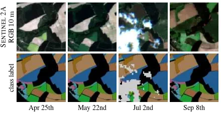
Figure 1. Sequence of observations during the growth season of the year 2016. SENTINEL2A RGB bands (top row) illustrate the
systematic and characteristic change of crops over the season. Class labels (bottom row) show the ground truth labels, as used for the training process. Coverage of the ground is considered by
additionalcoveredclasses, as shown ascloudsat July 2nd. The systematic temporal changes of spectral reflectances can benefit
identification of crops, as exploited by our proposed multi-temporal land cover classification network.
entire growth season of the year 2016, the effect of multi-temporal features has been evaluated by comparing the performance of multi-temporal models, namely LSTM networks and RNNs, with mono-temporalconvolutional neural network(CNN) models and asupport vector machine(SVM) baseline.
1.1 Remote Sensing of Phenology
plants change their reflective spectral characteristics which can be observed via remote sensing technologies. Phenological char-acteristics are assumed to change in a predictive manner and can thus be utilized for identification, as long as farming practices and environmental conditions remain unchanged or are considered in the model (Odenweller and Johnson, 1984; Foerster et al., 2012). Figure 1 illustrates reflective RGB responses of different crops in SENTINEL2A observations along the growth season. Fields containing the same types of cultivated crops change their spectral appearance uniformly within the series of observation. This is due to a combination of the crops phenological cycles and farming practices, such as the date of seeding and or harvesting.
Commonly, vegetation remote sensing usesvegetation indices— e.g.,thenormalized difference vegetation index(NDVI) or en-hanced vegetation index(EVI)—to observe these changes over a temporal series of observations (Reed et al., 1994). However, these indices usually consider only a limited number of bands which are predominantly sensitive to chlorophyll and water content,i.e., red and near infrared wavelengths. Further spectral bands are often discarded, even though that information is perceived by the satellite and may also contribute to the classification procedure. Additionally, these approaches need to filter high-frequent cov-erages, such as clouds, as preprocessing routines or by applying upper envelope filters(Bradley et al., 2007) to remove negative out-liers from the temporal profiles. Overall, these manually-crafted functional models might not be able to represent the complex ef-fects of various influencing factors—such as, for instance, weather conditions, sunlight exposure, or farming practices—which are encoded in the reflectance signal. For these reasons, very recent research has started to employdeep learningtechniques to over-come these limitations for crop yield prediction (You et al., 2017) and classification of phenological events (Ikasari et al., 2016).
2. RELATED WORK
Even though vegetation analysis with continuous monitoring over the growth season dates back many decades (Reed et al., 1994), only recently space-born sensors—namely the LANDSAT and ESA SENTINELseries—provide sufficientground sampling dis-tance(GSD) and temporal resolution for single-plot field clas-sification. Thus, classical land-cover classification approaches have concentrated on multi- or hyperspectral sensors at one single observation time. Matton et al. (2015) propose a generic methodol-ogy for global cropland mapping and statistical temporal features derived from LANDSAT-7 and SPOT images forK-meansand maximum likelihoodclassifiers on eight test regions on the entire world. Following this approach, Valero et al. (2016) use SEN -TINEL2A images to create a binary cropland/non-cropland mask by usingrandomized decision forests(RDF) classifiers on statis-tical temporal features extracted from spectro-temporal profiles. Foerster et al. (2012) make first attempts to utilize temporal infor-mation for per-plot identification by extracting spectro-temporal NDVI profiles and adjusting these profiles by additional agro-meteorological information to account for seasonal variations in phenology. They use LANDSAT-7 images aggregated over several years from a large study area in north-east Germany and classify twelve crop classes in total. While these approaches follow a generic feature extraction and classification pipeline, Siachalou et al. (2015) utilize ahidden markov model(HMM) approach which retains sequential consistency of multi-temporal observations on four LANDSAT-7 and one RAPIDEYEobservation of Thessalon´ıki, Greece in 2010. Methodically similar to ours, Lyu et al. (2016)
LSTM Cell
σ σ tanh σ
×
×
+
×
tanh
clt−1
hl t−1
hl−1
t
cl t
hl t
hl t
ft it gt ot
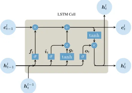
Figure 2. LSTM cells in layerlrecieve information of previous observations at time stept−1by means of two vectors: The hidden layerhlt−1represents the output information at previous
time and providesshort-term memory, similar to RNN cells. The cell state vectorclt−1carrieslong-terminformation. Based on the
forget gateft, information inctis discarded, inputitund modulationgtgates write new information toct. The updated
cell statectand the output gateotevaluate the hidden output layerhlt. (Figure adapted fromcolah.github.io/posts/
2015-08-Understanding-LSTMs)
utilize RNNs and LSTM architectures to multispectral LANDSAT -7 and hyperspectral EO-1 HYPERIONimages, but—in contrast to our approach—for the purpose of change detection.
3. METHODOLOGY 3.1 Neural Network Architectures
Traditional classification systems are assembled from sequential building blocks,e.g.,feature extraction, classification, and post processing, as summarized by ¨Unsalan and Boyer (2011). Fea-tures, which are expected to be significant for classification, are extracted from available observations,e.g., via estimating the parameters of functional models (Bradley et al., 2007). These features are further passed as inputs to classifiers like, for instance, maximum likelihoodclassifiers, SVMs, or RDFs. The optimal choice of feature extraction methodology and classifiers depends on the actual classification task and available data.
In contrast to these approaches,artificial neural networks (NNs) are trained in anend-to-endmanner, solely based on rawinput datax∈Rnandoutput labelsyˆ∈Rc. NNs are usually used for supervised learning to approximate non-linear response functions, e.g.,class probabilities, by a sequence of affine transformations
Wdata·x+bpassed to (usually non-linear) activation functions σ : Rm
7→ Rm
, e.g.,sigmoid or tangent functions. A loss functionquantifying the divergence between predicted and actual class probabilities is minimized at each training step by back-propagating residuals and adjusting the network weightsWdata∈
Rn×m
and biasesb ∈ Rm. Neural networks are commonly arranged in multiple stackedlayerswith the hidden output of one layer forming the input of the consecutive layer. Thenumber of neurons, expressed as dimensions of hidden vectorsmandnumber of layersl, are common hyper-parameters of which the optimal combination is determined based on classification performance on anvalidationdataset distinct from the training data corpus.
x1
t1
LSTM
softmax
ˆ
y1
H1( ˆy1,y1)
y1
x2
t2
LSTM
softmax
ˆ
y2
H2( ˆy2,y2)
y2
x3
t3
LSTM
softmax
ˆ
y3
H3( ˆy3,y3)
y3
input dataxt:
day of observationtt and raster reflectancesρt
network
predicted class probabilitiesyˆt
cross entropy loss
reference class probabilitiesyt
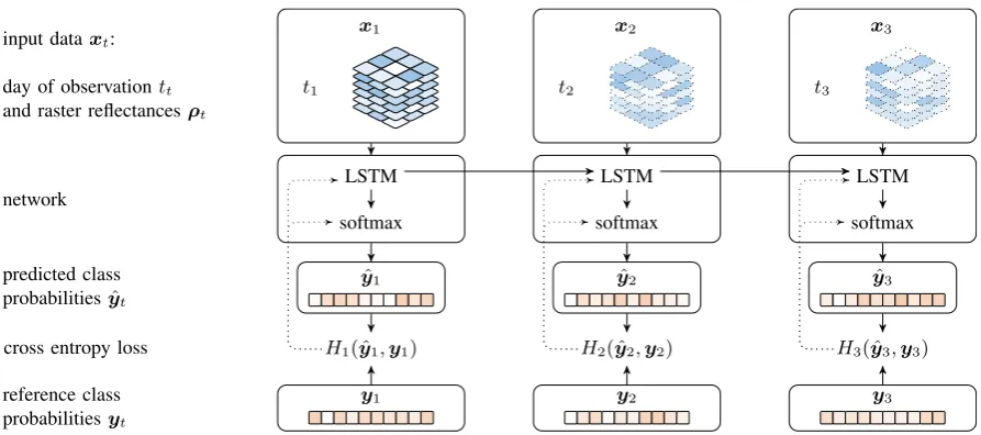
Figure 3. Unrolled flow of data for classification and training. Class probabilitiesyˆtare calculated by multiple stacked LSTM layers and one softmax layer. LSTM layers have additional access to cell state vectorsct−1andht−1originating from previous observations,
indicated by an arrow between processing columns, which benefits extraction of temporal features. At each training step, thecross entropy lossHt( ˆyt,yt)between predicted and reference class probabilites is calculated. To minimize the loss function, gradients
(dotted) are calculated by Adam optimizer and adjust the network weights in involved in LSTM and softmax layers.
important for classification based on available data. This scheme ensures that neural network architectures can be applied to a va-riety of tasks and scenarios, as long as a sufficient quantity of training data is available. Additionally, information which is not important for classification can be gradually ignored by the net-work. Hence, all available information can safely be provided to the deep learning model. Nevertheless, various neural network architectures have been developed for application to certain fields which—by design—excel at some types of features.
Mono-temporal models Feed-forward neural networksprocess input datain a one-directional pipeline. Image processing and segmentation feed forward neural networks incorporate additional convolutionallayers to account for local neighborhoods and thus are well suited for recognition of shapes and textural patterns. Due to these properties,convolutional neural networks(CNNs) are already applied in earth observation for high resolution satellite imagery (Hu et al., 2015) or semantic segmentation (Castelluccio et al., 2015).
Multi-temporal models RNNs (Werbos, 1990) are potentially well suited for processing sequential data, such as temporal se-quences of observations, as the network has access to information of the previous observation for the classification of current obser-vation. At each network layerland observationt, a hidden output vectorhltis derived from the output of the previous observation
hlt−1and the input of the current observationh
l−1
t . Hence, deci-sions can be based on thecontextof previous observations, thus making RNNs a useful architecture for language processing, text generation, or voice recognition.
Inducing a further level of complexity,long short-term memory (LSTM) networks (Hochreiter and Schmidhuber, 1997) introduce an additionalcell state vectorclt ∈ R
m
providing long-term memory capabilities, as at each observationtinformation can be stored or retrieved to varying extents. Figure 2 illustrates the flow of vectorized information within one LSTM cell layerl. At each observationt, the previous cell state vectorcl
t−1is manipulated
by a set of gates,i.e.,theforget gateftlfor discarding information and theinput gateil
tcombined with themodulation gateg l tfor
writing additional information tocl
t. The output gateo l
tis derived based onhlt−1andh
l−1
t and provides the same functionality as a RNN layer. The new output vectorhl
tis then obtained by an element-wise multiplication of the output gateolt and the cell stateclt. While our approach is based on these LSTM networks (Zaremba et al., 2014), a variety of variations have been presented in the past (Gers et al., 2002; Graves and Schmidhuber, 2005; Graves et al., 2013; Kalchbrenner et al., 2015).
3.2 Approach
We employ LSTM neural networks for the purpose of crop clas-sification on a per-plot scale from medium resolution satellite imagery. Figure 3 illustrates the classification and training scheme of our approach for at multiple consecutive observations. At each observationt,nsspectralbottom-of-atmospherereflectance mea-surementsρi∈R(
k×k)·ns
, along with the day of observationti are fed to the network as input vectorx. A series oflLSTM layers process the data with additional information of the previous observationt−1. Asoftmaxlayer produces probabilities for each classyˆt. At each training step, thecross-entropy losswrt. predicted and actual class probabilities is calculated. Gradients are calculated byAdamoptimizer (Kingma and Ba, 2014) and back-propagated in order to adjust the network weights.
Crops have been chosen as subject of classification since these land cover classes are expected to change in a characteristic manner, as explained in Section 1.1, thus making these classes ideal subjects to demonstrate the capabilities of temporal modeling by LSTM networks.
4. EXPERIMENTS
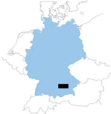
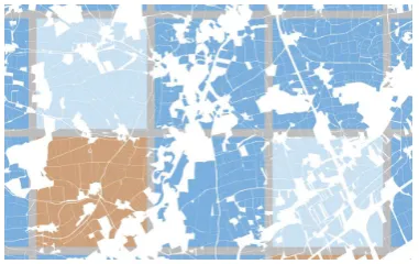
Figure 4. In our experiments, we used anarea of interestof
102 km×42 km(black rectangle) in the north of Munich,
Germany, as study area containing137 kfield plots.
obtained data in Section 4.1 and the performed data aggregation to obtain input and label vectors in Section 4.2. Section 4.3 explains the intuitions behind the different dataset partitioning regimes to obtaintraining,validation, andevaluationsubsets in the context of phenological temporal features and regional en-vironmental influences. The training and evaluation process is explained in Section 4.4 and results are shown in Section 4.5.
4.1 Data Material
To train the large number of neural network weights, a feasible body of raster and label data is necessary. For this reason a large area of interest(AOI) of102 km×42 kmin the north of Munich, Germany, has been selected (cf.Figure 4) due to its homogeneous geography, climate conditions, and farming practices which sug-gest similar environmental conditions. Arasterdataset of 26 SENTINEL2A images, acquired between 31stDecember, 2015 and 30th September, 2016, has been retrieved from ESA SCI -HUBand atmospherically corrected by SEN2CORsoftware. For consistency reasons with the LANDSATseries,blue,green,red, near-infraredandshortwave infrared 1and2bands were selected for this evaluation. Field geometries and cultivated crop labels of
137 kfields in the AOI have been provided by theBavarian
Min-istry of Agriculture(Bayrische Staatsministerium f¨ur Ern¨ahrung, Landwirtschaft und Forsten).
The distribution of fields per crop class is not uniform with com-mon cultivated crops,e.g.,cornorwheat, dominating the dataset, while other crops,e.g.,sugar beetorasparagus, are less repre-sented (cf.Figure 5). Nevertheless, from 172 unique field crops, 19fieldclasses have been selected with at least 400 field-plots in the AOI.
4.2 Data Extraction
The field geometries of thefieldand reflection values of the rasterdataset have been discretized to a100 m×100 mgrid ofpoints of interest(POIs). Each POI contains information of network input xand classification ground truth labels y in a 30 m×30 mneighborhood. The network input vectorx incor-poratedbottom-of-atmospherereflection values directly derived from therasterdataset combined with the day of observation
othercorn meado
w
asparagus rape hop
summer oats
winter speltfallow
winter wheat
winter barle
y
winter rye
beans
winter triticale
summer barle
y peas
potatoesoybeans sugar
beets 0
.001 0
.01 0
.1
crop class
frequenc
y
Training examples Testing examples
Figure 5. Distribution of classes by fields in the AOI. Common field crops, such ascornorwheat, dominate the dataset with 28k
and 22k fields, respectively, while,e.g.,asparagusorpeasare cultivated in less than 600 fields. Only crops with at least 400
occurances have been included in the dataset.
normalized asfraction of year. The network labelsyhave been formed by two types of classes.
1. Fieldclasses were derived from thefielddataset, namely
corn,meadow,asparagus,rape,hop,summer oats,winter spelt,fallow,winter wheat,winter barley,winter rye,beans,
winter triticale,summer barley,peas,potatoe,sugar beets,
soybeans, and the default classother.
2. Coveredclassescloud,water,snow, andcloud shadow, ac-count for high frequent coverages and are provided by the scene classification maskof SEN2CORextracted from the rasterdataset.
If POIs were located at the border of multiple classes, class labels have been weighted with respect to a local30 mneighborhood.
4.3 Dataset Partitioning
Commonly, two sets of parameters need to be determined when selecting and training the neural network architecture. Weights
W ∈ Rn×m
are adjusted during the training process by back-propagation of residuals andhyper-parametersθare chosen fol-lowing a grid search regime in order to find the optimal network structure for the classification task. To ensure that these param-eters are chosen independently, training of network weights and evaluation of hyper-parameters was performed ontrainingand validationdatasets, respectively. A thirdevaluationdataset is used for to calculate accuracy measures of neural network independently from network weights and parameters. While theevaluationdataset remained unchanged, training and validationwere redistributed in multiplefolds. This practice maximizes the number of training samples and avoids misrepre-sentations of classes containing small numbers of features in the respective dataset. Hence, the body of POIs was divided in the three respective datasets.
As discussed in Section 1.1, the dates of phenological events are influenced by environmental conditions which vary at large spatial distances. To average these environmental conditions, the body of data is divided randomly with respect to the extent of the AOI. A pure random assignment of individual POIs would ensure an even distribution of POIs but may assign POIs of the same field to the different datasets and thus cause dependencies between datasets.
Figure 6. Illustration of thefielddataset overlayed with 3 km×3 kmblocks dedicated fortraining(blue), evaluation(lightblue), andvalidation(orange). A circumferential margin of200 mensures that field plots are not
located in two distinct datasets.Trainingandevaluation datasets are randomly reassigned at each cross-validationfold.
blocks. These 476 blocks of3 km×3 kmwere in turn randomly assigned totraining,validation, andevaluationin a 4:1:1 ratio (cf. Figure 6). A circumferential margin of200 mensures that POIs located on the same field were not assigned to differ-ent datasets. At eachfold,trainingandevaluationblocks got reassigned randomly while thevalidationdataset remained unchanged.
4.4 Experimental Setup
In total, 135 networks of each architecture have been trained the body oftrainingdata over 30 epochs with varying hyper-parameters l ∈ {2,3,4}andr ∈ {110,220,330,440,880}. This process has been repeated in 9 folds of randomly reassigned trainingandvalidationdatasets. Dropout with probability pdropout= 0.5was used for regularization. Additional to the inves-tigated neural network architectures, a baseline SVM withradial basis function(RBF) kernel was trained on a balanced dataset of 3,000 samples per class extracted from thetrainingdataset. The optimal hyper-parameters,i.e., slack penaltyC and RBF scaling factorγ, have been chosen based on a grid search over C ∈
10−2, ...,106 andγ ∈
10−2, ...,103 . All networks
have been trained within 8 hours on a NVIDIA DGX-1 server equipped with eight NVIDIA TESLAP100 GPUs and16 GB VRAM each. Five networks have been able to be trained on each GPU in parallel, making the large grid search of parameters possi-ble. While neural networks were implemented in TENSORFLOW, the SVM baseline based on theSCIKIT-LEARNframework.
The best network performances have been achieved by networks with hyper-parameter settingsθLSTM= (l= 4, r= 440),θRNN= (4,880), andθCNN= (3,880). The SVM baseline performed best
withθSVM= (C= 10, γ= 10).
4.5 Results
In this section, we evaluate the performance of the trained net-works at multiple scales from general performance of each neural network architecture to the performance of best networks on indi-vidual classes.
4.5.1 Training performance Figure 7 shows the overall ac-curacy of each architecture on thevalidationdataset within the training process by means of the average overall accuracy as indication of general performance of the respective architecture. Variations of observed accuracy were presumably caused by the
0 2 4 6
·106
0.5
0.6
0.7
0.8
0.9
training iterations
o
v
erall
accurac
y
CNNσ CNN mean CNN best RNNσ RNN mean RNN best LSTMσ LSTM mean LSTM best
Figure 7. Evolution of overall validation accuracy performance during the training process of 135 networks of each CNN, RNN,
and LSTM architecture with different hyperparameter settings. Means (dashed lines) and standard deviation intervals (shaded areas) indicate the general performance of each architecture, the most performand network is superimposed separately (solid line).
chosen hyper-parameter sets and are indicated by their standard deviation intervals. These standard deviations turned out to be rel-atively small compared to the performances of LSTM, RNN, and CNN models and suggest that, on this dataset, the choice of the ac-tual architecture has larger influence on classification performance than the choice of the involved hyper-parameters. Overall, LSTM networks and RNNs achieved significantly better accuracies over the entire training process with LSTM models performing slightly better than their RNN competitors. The networks which achieved best accuracies are plotted separately as solid lines, as these will be evaluated in detail in the following.
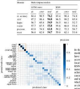
4.5.2 Accuracy measures per best network The best per-forming networks, opposed to the SVM baseline, have been tested in detail on theevaluationdataset. Results of these experiments are compiled in Table 1. Additionally,coveredandfieldclasses have been separated from each other. Similarly to the previous fig-ure, multi-temporal models achieved better accuracies compared to mono-temporal competitors. This performance gain is supposed to be largely caused by thefieldclasses which—in contrast to cov-eredclasses—contain temporal phenological characteristics likely to be utilized by LSTMs and RNNs. Covered classes achieved similar accuracies in all of the models with also the baseline SVM achieving good classification accuracies. Apparently, the charac-teristics of these classes are more distinctive and can be utilized by all models.
4.5.3 Class confusions Similar results can be observed from the confusion matrices shown in Figure 9 based on the best per-forming networks and the SVM baseline shown in Figure 8. The class frequencies are normalized by the sum of ground truth classes to obtain the precision measure. While some classes represent distinct cultivated crop, other classes—such asmeadow,fallow, or
Table 1. Performance evaluation of our proposed LSTM-based method in comparison to standard RNNs and mono-temporal baselines based on CNNs and SVMs. Ascoverclasses (i.e.,,cloud,cloud shadow,water, andsnow) are usually comparatively easy to recognize,
we restrict our evaluation to unbiased performance measures with respect to the remainingfieldclasses,
Measure Multi-temporal models Mono-temporal models
LSTM (ours) RNN CNN SVM (baseline)
all cover field all cover field all cover field all cover field
ov. accuracy 84.4 98.5 76.2 83.4 98.4 74.8 76.8 98.4 59.9 40.9 90.4 31.7 AUC 97.2 99.4 96.8 96.5 99.2 95.9 91.7 99.3 90.2 87.1 98.9 84.8 kappa 56.7 65.8 54.9 54.5 64.1 52.7 28.6 61.9 22.2 34.3 83.2 24.9 f-score 57.7 67.5 55.8 55.6 66.0 53.6 30.1 64.3 23.6 40.3 85.0 31.7 precision 63.8 74.8 61.8 59.2 72.3 56.7 47.3 69.1 42.2 40.3 83.1 32.2 recall 56.0 62.8 54.7 55.0 62.1 53.6 29.1 61.4 22.9 40.6 87.4 31.7
cloud water snow cloud shadow other corn meadow asparagus rape hop summer oats winter spelt fallow winter wheat winter barley winter rye beans winter triticale summer barley peas potatoe soybeans sugar beets
predicted class
ground
truth
class
0 0 .2 0
.4 0
.6 0
.8 1 precision
Figure 8. Confusion matrix of SVM classification. Whilecovered
classes, indicated by theorange-framed submatrix, have been classified well,fieldclasses were confused broadly.
while others have not been classified at all or got interchanged with classes showing particular spectral similarities. Presumably the spectral characteristic of some crops are distinct enough for classification without temporal information, while other crops are not distinguishable solely by spectral features. The SVM model showed broad confusion for allfieldclasses which indicates that this classifier does not provide a sufficient amount of capacity to encode detailed crop-specific characteristics. SVM, though, performed especially well on thecovered classes, of which the spectral characteristics are more distinctive.
4.5.4 Accuracy over sequence of observation As LSTM and RNN networks utilize additional information of previous observa-tions, accuracy is expected to improve with increasing sequence length. Figure 10 illustrates this relationship, where the recall values onfieldclasses of the three respective networks were cal-culated by day of observation. While all models, in general, per-formed equal during the first couple of observations, the accuracy of LSTM and RNN models increased with the sequence of obser-vations. The later the observation is registered, the more context information is available to the temporal models to evaluate the classification decision. The performance of temporal models in-creases especially at the beginning of vegetation period between March and April (day of year 100), likely due to characteristic phenological events. This trend continues to late summer, up to which crops are harvested, and fields are prepared for the next season, which may cause the slight decrease by the end of growth season.
5. DISCUSSION
In this work, we have shown how to employ LSTM and RNN models for land cover classification. Large-scale experiments have been conducted on a real-world dataset acquired from open-access satellite data together within-situannotations provided by local authorities. These experiments have shown that LSTM and RNN networks are able to directly utilize temporal information, namely phenological characteristics of crops, for classification and achieve superior results compared to models which—by design— can not benefit from these features but solely rely only on spectral and textural characteristics. All models performed well on classes which do not incorporate characteristic temporal information, such as clouds, while crops can be reliably better classified by LSTM networks and RNNs utilizing distinct phenological events.
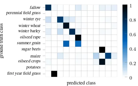
Our LSTM model achieved good classification accuracies com-pared state-of-the art, while considering a notably larger number of crop classes (Foerster et al., 2012; Siachalou et al., 2015). While thehidden markov modelapproach of Siachalou et al. (2015) is methodically closest to our deep learning strategy, their relatively small study area together with their small number of classes im-pede direct comparison. Our deep learning approach achieved better accuracy performance than the approach of Foerster et al. (2012) using spectro-temporal NDVI profiles and adjusting these by additional agro-meteorological information (cf. Figure 11). Their considerably large test area is located in north-east Germany and fields are comparable with ours in terms of cultivated crops and farming practices. Hence, their work is most comparable in terms of data.
In this work, LSTM and RNN architectures have been shown to perform similar, with the LSTM model achieving slightly better accuracies consistently over all evaluation schemes. With increas-ing observation length, LSTM models may be able to exhaust their full long-term memory capabilities which may be advantageous for monitoring multiple years or data with a higher temporal fre-quency. As a side effect, the LSTM model have learnedcloud
andcloud shadowdetection along with field classifications with good overall accuracy of98.5%by providing additionalcovered
cloud
Figure 9. Confusion matrices reporting class-wise average accuracy values of LSTM, RNN, and CNN architectures. Theorange-framed submatrix comprisescoveredclasses. While LSTM and RNN showed similarily good performances, as these networks utilize temporal features, the CNN network performed generally worse, as temporal characteristic features are not accessible to the CNN architecture.
0 50 100 150 200 250
Figure 10. Evolution of performance of LSTM, RNN, and CNN networks with increasing number of observations. The more observations have been registered, the more context information
was available to multi-temporal LSTM and RNN networks to assist the classification decision. CNN models can not utilize temporal information, thus performance remained at a nearly
constant level with increasing observation length.
6. CONCLUSIONS
Many applications and architectures of thedeep learning com-munity can be applied to the domain of earth observation for efficient, large scale data processing. This work has demonstrated the applicability oflong short-term memory(LSTM) networks, originating from speech and text generation, for earth observation. Earth observation, in particular, has to face increasing amounts of data from a variety of multi-modal sensors, such as the SENTINEL, LANDSAT, or MODIS satellite series. The acquired information needs to be processed on a large scale and in an efficient manner ex-ploiting all available information. Considering these requirements, neural networks provide flexibility in terms of preprocessing and provided data, as,e.g.,no cloud filtering is necessary if the net-work has been trained on additionalcloudclasses. Additionally, data which is not significant for the given task will be ignored. We believe that a holistic data approach—comprising temporal, spec-tral, and textural information—has the potential to yield superior results in future applications. Our presented approach limits textu-ral and spatial features by only observing a small neighborhood of 30 maround each POI to concentrate on available temporal
infor-fallow first year field grass
predicted class
Figure 11. Confusion matrix reporting class-wise average accuracy values reported by Foerster et al. (2012).
mation. In future work, a CNN encoder prepended to the LSTM network could additionally benefit the classification accuracy, as richer textural features would be extracted in a perceptive field optimally chosen by the network.
7. ACKNOWLEDGEMENTS
We would like to thank the Bavarian Ministry of Agriculture for providing information of cultivated crops in high geometrical and semantic accuracy. The TITANX PASCALused for this research was donated by the NVIDIA CORPORATION.
References
Bradley, B. A., Jacob, R. W., Hermance, J. F. and Mustard, J. F., 2007. A curve fitting procedure to derive inter-annual phe-nologies from time series of noisy satellite ndvi data.Remote Sensing of Environment106(2), pp. 137–145.
Castelluccio, M., Poggi, G., Sansone, C. and Verdoliva, L., 2015. Land Use Classification in Remote Sensing Images by Convo-lutional Neural Networks. arXiv preprint arXiv:1508.00092 pp. 1–11.
Gers, F. A., Schraudolph, N. N. and Schmidhuber, J., 2002. Learn-ing precise timLearn-ing with lstm recurrent networks. Journal of machine learning research3(Aug), pp. 115–143.
Graves, A. and Schmidhuber, J., 2005. Framewise phoneme classification with bidirectional lstm and other neural network architectures.Neural Networks18(5), pp. 602–610.
Graves, A., Mohamed, A.-r. and Hinton, G., 2013. Speech recogni-tion with deep recurrent neural networks. In:Acoustics, speech and signal processing (icassp), 2013 ieee international confer-ence on, IEEE, pp. 6645–6649.
Hochreiter, S. and Schmidhuber, J., 1997. Long Short-Term Memory.Neural Computation9(8), pp. 1735–1780.
Hu, F., Xia, G.-S., Hu, J. and Zhang, L., 2015. Transferring Deep Convolutional Neural Networks for the Scene Classification of High-Resolution Remote Sensing Imagery. Remote Sensing 7(11), pp. 14680–14707.
Ikasari, I. H., Ayumi, V., Fanany, M. I. and Mulyono, S., 2016. Multiple regularizations deep learning for paddy growth stages classification from landsat-8.arXiv preprint arXiv:1610.01795.
Kalchbrenner, N., Danihelka, I. and Graves, A., 2015. Grid long short-term memory.arXiv preprint arXiv:1507.01526.
Kingma, D. and Ba, J., 2014. Adam: A method for stochastic optimization.arXiv preprint arXiv:1412.6980.
Lyu, H., Lu, H. and Mou, L., 2016. Learning a Transferable Change Rule from a Recurrent Neural Network for Land Cover Change Detection.Remote Sensing8(6), pp. 1–22.
Matton, N., Canto, G. S., Waldner, F., Valero, S., Morin, D., Inglada, J., Arias, M., Bontemps, S., Koetz, B. and Defourny, P., 2015. An Automated Method for Annual Cropland Mapping along the Season for Various Globally-Distributed Agrosys-tems Using High Spatial and Temporal Resolution Time Series. Remote Sensing7(10), pp. 13208–13232.
Odenweller, J. B. and Johnson, K. I., 1984. Crop identification using landsat temporal-spectral profiles. Remote Sensing of Environment14(1-3), pp. 39–54.
Reed, B. C., Brown, J. F., VanderZee, D., Loveland, T. R., Mer-chant, J. W. and Ohlen, D. O., 1994. Measuring Phenologi-cal Variability from Satellite Imagery. Journal of Vegetation Science, 5(5), 703–714. http://doi.org/10.2307/3235884suring Phenologica.Journal of Vegetation Science5(5), pp. 703–714.
Siachalou, S., Mallinis, G. and Tsakiri-Strati, M., 2015. A Hidden Markov Models Approach for Crop Classification: Linking Crop Phenology to Time Series of Multi-Sensor Remote Sens-ing Data.Remote Sensing7(4), pp. 3633–3650.
¨
Unsalan, C. and Boyer, K. L., 2011. Review on Land Use Classifi-cation. In:Multispectral Satellite Image Understanding: From Land Classification to Building and Road Detection, Springer, pp. 49–64.
Valero, S., Morin, D., Inglada, J., Sepulcre, G., Arias, M., Hagolle, O., Dedieu, G., Bontemps, S., Defourny, P. and Koetz, B., 2016. Production of a Dynamic Cropland Mask by Processing Remote Sensing Image Series at High Temporal and Spatial Resolutions. Remote Sensing8(1), pp. 1–21.
Werbos, P. J., 1990. Backpropagation through time: what it does and how to do it.Proceedings of the IEEE78(10), pp. 1550– 1560.
Whitcraft, A. K., Becker-Reshef, I. and Justice, C. O., 2014. Agri-cultural growing season calendars derived from MODIS surface reflectance.International Journal of Digital Earth8(3), pp. 173– 197.
You, J., Li, X., Low, M., Lobell, D. and Ermon, S., 2017. Deep gaussian process for crop yield prediction based on remote sensing data.