ROAD DETECTION BY NEURAL AND GENETIC ALGORITHM IN URBAN
ENVIRONMENT
A. Barsi*
Dept. of Photogrammetry and Geoinformatics, Budapest University of Technology and Economics, Budapest, Hungary – barsi@eik.bme.hu
Commission III, WG III/4
KEY WORDS: Segmentation, Genetic algorithm, Differential evolution, Road detection
ABSTRACT:
In the urban object detection challenge organized by the ISPRS WG III/4 high geometric and radiometric resolution aerial images about Vaihingen/Stuttgart, Germany are distributed. The acquired data set contains optical false color, near infrared images and airborne laserscanning data. The presented research focused exclusively on the optical image, so the elevation information was ignored. The road detection procedure has been built up of two main phases: a segmentation done by neural networks and a compilation made by genetic algorithms. The applied neural networks were support vector machines with radial basis kernel function and self-organizing maps with hexagonal network topology and Euclidean distance function for neighborhood management. The neural techniques have been compared by hyperbox classifier, known from the statistical image classification practice. The compilation of the segmentation is realized by a novel application of the common genetic algorithm and by differential evolution technique. The genes were implemented to detect the road elements by evaluating a special binary fitness function. The results have proven that the evolutional technique can automatically find major road segments.
* Corresponding author.
1. INTRODUCTION
The working group III/4 of ISPRS Commission III has conducted a challenge of detecting man-made objects from digital aerial imagery. These objects are urban objects (roads, trees, cars etc.) and 3D buildings. This challenge has been supported by adequate data sets: there was an aerial photography campaign near Stuttgart, Germany, when color images and LIDAR-point clouds were acquired. The raw data were processed: the aerotriangulation was calculated, and digital elevation model (DEM) was derived. All of these products can be downloaded and used for developing object detection methodologies.
The author is strongly interested in the use of current developments of computer science in digital image understanding. Among the modern methods neural network based classification techniques and genetic algorithms can be mentioned, which are in the focus of the current paper.
The general theory of the two artificial intelligence tools is presented, followed by the details of the applied methodology in image analysis.
2. NEURAL AND GENETIC ALGORITHMS
2.1 Neural networks as classifiers
The artificial neural networks have become widely used tool in different data processing workflows, among them also in digital image processing. There are several types of network; therefore different categorization can be done, for example
by the architecture (layers, recurrent, delay, transfer functions etc.),
by the initialization, training, testing and validation algorithms,
by the data structure and configuration,
by the used pre- and post-processing operations. The most used neural networks in image processing have a strong focus on classification, which is appropriate application for back-propagation (BP) network, radial basis function (RBF) networks, learning vector quantization (LVQ) networks and support vector machines (SVM). Beside these supervised classifiers, the unsupervised category is similarly important: e.g. self-organizing maps (SOM), competitive learning networks. [Beale et al, 2012]
The current paper presents applications of SVM and SOM technologies. The used support vector machine classification is based on the formula:
s x bk c
i i
i
,(1)
where siis the support vector, x is the vector to be classified,
k is the kernel function, iis a weight, b is a bias, and c is the result, which having a value more than zero means to be classified in the category, otherwise it is rejected. The applied kernel function was the radial basis function (RBF), which is a nonlinear function, so it has the advantage to make right decision even with complicated class borders. This supervised classification method must be parameterized by data from training areas [Beale et al, 2012].
The T. Kohonen developed SOM is a widely used unsupervised data clustering technique, also in image processing. It has a competitive learning algorithm combined with a topologically ordered neuron structure, where the input vector has been compared with all neurons, then the weights of the winner and its neighboring neurons must be increased. At the end the neurons will split the data space, so clusters are built.
2.2 Genetic algorithms
The genetic algorithms (GA) are tools based on artificial reproduction of the evolution theory. The elements are the genes (chromosomes), which encode the relevant information of the studied phenomena. The simultaneously handled genes build the population, where – similarly to the real world biology
– two rules must take their effect:
mutation, which alters the encoded information in the
genes, and genes can be sorted by their fitness value and depending of the control procedure the last items can be removed from the population (delete). Some authors extend this list by two more operations, namely selection and inheritance.
All these steps called an epoch (generation) must be repeated several times. In ideal case the fitness of the whole population and therefore also of the best gene will converge to an optimum, which can be a minimum or a maximum. One big advantage of
the technology is that it doesn’t require monotonic and/or differentiable fitness function; it can be used even with discrete, complex, non-monotonic fitness surface having discontinuities. Its disadvantages are the hard control or the possible long run (with high computation efforts).
2.3 Differential evolution
The alternative name of the genetic algorithms is the evolutionary algorithms. There is a new differential evolution (DE) method developed by R. Storn and K. Price, which is based on strong improving of randomly selected genes by comparing further independent genes. This algorithm belongs to the metaheuristic search methodology; it is able to evaluate huge spaces of candidate solutions, but as a drawback it doesn’t always guarantee whether the optimum is found.
The basic steps of the DE technique are the following [Laky, mutation is easily calculated by the following formula:
jG kG
vectors representing the n-dimensional data encoded within the gene.The mutation is followed by the crossover using the formula:
The selection step means that the successor has been compared to its predecessor by their fitness values and the one having better value will survive and the other is removed.
The differential evolution runs till the given epoch number has been reached.
There are further variations in combining the genes, as well as according to the used selection algorithm.
3. ROAD DETECTION METHODOLOGY
3.1 Data set of the pilot area
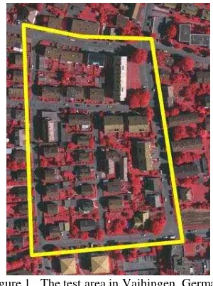
The used data set covers Vaihingen, near Stuttgart, Germany. The images were taken from the earlier digital camera test of the German Association of Photogrammetry and Remote Sensing (DGPF). The images were captured by a Z/I Intergraph DMC camera on 24 July and 6 August 2008. The block consisted of five overlapping strips with two additional cross strips at both ends of the block. The flying height was about 900 m, the focal length of the camera was ~120 mm. The ground sampling distance (GSD) was 8 cm, the radiometric resolution was 11 bits, but the provided TIFF-images have 16 bit color depth. The sensors have captured the near-infrared, the red and the green channels (false color composite). On August 21, 2008, LIDAR data were also acquired by a Leica ALS50 system, but these
data weren’t used in the current investigation. The laser scanning flying height was about 500 m and had a point density of 4 points/m2. The test area can be seen in Fig. 1. [Rottensteiner et al, 2011]
Figure 1. The test area in Vaihingen, Germany
The applied image has a size of 3145 by 2436 pixels, that is – regarding the GSD –a pilot area of 252 × 195 m.
3.2 The developed workflow
The urban scene of the pilot area contains several roads and streets. There are also cars and shadows of the trees or buildings, which disturb the exact recognition of the roads. An idea to overcome on this difficulty was to implement a two phase workflow, where the first phase – the segmentation – extracts pixel candidates belonging possibly to road category, then a sophisticated linkage (detection) can compile the final roads. The resulting binary image of the first step unfortunately contains wrongly road classified pixels; in some cases only scattered points build these noisy pixels. To remove these pixels a median filter has been applied.
The linking phase itself has two subphases: the first one is an automatic, while the second requires human interaction. Because the automatic compilation step has the genetic
3.3 Segmentation of the imagery
The first segmentation method was the support vector machine, which needs suitable training areas. Four road training sites were marked; the total area was 5726 pixel, means 36.6 m2, which is 0.8% of the covered image. The training data set was extended with non-road pixels of the same amount.
The SVM-classification starts with training, where the network parameters are to be determined. After several experiments with linear and RBF kernels, it came out that the size of the data set is too big, so a resampling had to be executed. The kept data set had 1769 road and non-road pixels, where the ratio was 64.8%-35.2%.
As only the image intensity information was to be used for the classification, a scatterplot analysis was performed. Because of the strong overlapping, two ways were open:
extend the information by additional sources,
decorrelate the groups by mathematical techniques (e.g. principal component analysis).
The additional information source intended to be kept in relation with the image, i.e. the use of elevation information was rejected. Image base additional sources can then be for example the vegetation indices. The normalized differential vegetation index (NDVI) is also defined for aerial (and ortho) images; a small modification increased our accuracy:
B
The calculated NDVI was added as the fourth dimension. The decorrelation by the principal component analysis (PCA) and transformation is also a frequently used preprocessing step before neural classification. The result of the repeated scatter analysis can be seen in Fig. 2.
The RBF kernel function can be controlled by its sigma scaling factor, whose value was at first strongly increased to produce any result, then was successively decreased to get better classification accuracy.
The classification accuracy was measured in this context as in-sample accuracy, meaning the trained network was used to classify only the training data set. The overall accuracy (OA)
was sufficient to evaluate which setting leads to the best performance.
Figure 2. Decorrelated inputs for SVM training with road (red dots) and non-road (blue dots) samples
The SOM segmentation needs no training data, but the definition of the layered neurons. After initial tests a 9×9 neuron sized hexagonal mesh was accepted with Euclidean distance measure. The training was set with 200 epochs, having the whole image as inputs.
To be able to compare both described classification method, a third type was also done: a hyperbox (parallelepiped) classification, known from the statistical pattern recognition. This supervised method was fed by parameters derived from the already mentioned training sites. The box-classifier parameters were the intensity minimum and maximum values in each image bands.
All these presented segmentation techniques resulted a binary thematic map with road and non-road pixels. The binary images were given to the genetic algorithms in the next processing phase.
3.4 Detecting road segments
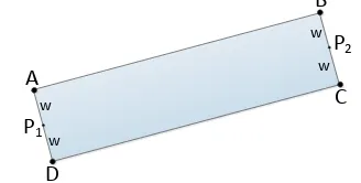
The genes as road segments are defined by rectangles, where the key points are the two midpoints (P1 and P2) of the shorter
Figure 3. Definition of the basic road segment by rectangle
The population is built up of these rectangles. During the initialization 50-100 rectangles were generated with random coordinates for points P1 and P2, where the width parameter w was fixed. The rectangles are masks laid on the binary segmentation image. The fitness function can be defined for this binary subimage, as follows
counting the covered road pixels,
based on the number of the covered road pixels divided by the length/area of the rectangle,
calculating ratio of the road and non-road pixels
divided by the rectangle’s area, weighted by the reciprocal logarithm of the road pixels.
The genetic algorithm technology needs a suitable fitness definition, but all of the above mentioned have practical considerations. The first fitness optimization is a maximum search, but globally all road pixels can be categorized also by small rectangles (short road segments). The second fitness definition fixes this problem by a length/area based weighting, but behaves too rough and converges drastically into a single rectangle state. The last definition was found as the best (Eq. 5).
maskpixels
where the # operator means the number of pixels. The logarithm can be also the natural logarithm function. This fitness function supports the minimum search optimization.
Other, similarly suitable fitness functions can be defined and their performance has to be evaluated.
The listed fitness functions can be implemented not only considering genetic algorithms, but with differential evolution, too.
The execution of the automatic road segment compilation must be followed by a human evaluation and network creation.
4. RESULTS
4.1 Segmentation results
The support vector machine training results a support vector set of 1701 elements. The training lasts 140 s, thereafter the classification of the whole image requires only 56 s. The in-sample confusion matrix is as follows:
Roa d Non-roa d Σ OE PA
Roa d 1146 0 1146 0,00% 100,00%
Non-roa d 142 481 623 22,79% 77,21%
Σ 1288 481 1769
Table 1. In-sample accuracy for SVM classifier
The overall accuracy is 91.97%, the average accuracy is
88.60%, the accuracy of road recognition (producer’s accuracy)
is 100%. The output image is visually not satisfactory, because a lot of roof pixels are also ordered to the road category. The SOM solution has produced a label image containing 9 different label values. The most similar label images are the 5th and 8th, so their union is handled as road category. The confusion matrix was derived in the same way (Table 2). As one can see, the overall accuracy is less, than before: 89.77%, the average accuracy is similarly lower: 85.55%. The hyperbox method was the last classification algorithm, which was also evaluated. This technique is very fast, because the relational operations are of very low level, so they can be executed quickly. The error matrix is in Table 3.
The average accuracy is the highest at this method, it is 91.97%, the overall accuracy is very close to this value with 91.63%.
Non-roa d 179 444 623 28,73% 71,27%
Σ 1323 446 1769
Table 2. In-sample accuracy for SOM classifier
Σ OE PA
Roa d Non-roa d OE PA
Roa d 1041 105 1146 9,16% 90,84%
Non-roa d 43 580 623 6,90% 93,10%
Σ 1084 685 1769
Table 3. In-sample accuracy for hyperbox classifier
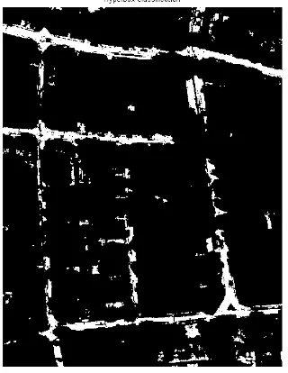
The best binary result (Fig. 4) of the hyperbox algorithm therefore was propagated into the next phase.
Figure 4. Result of the segmentation by the hyperbox technique
Since the segmentation results were not fully satisfactory, and the genetic algorithm was intended to be tested, a set of synthetic images were created. These synthetic images contain only binary pixels labeling the road pixels.
4.2 Road detection results International Archives of the Photogrammetry, Remote Sensing and Spatial Information Sciences, Volume XXXIX-B3, 2012
in these cases 30-50 pixels were set. The fitness function was at the beginning only the correctly detected road pixels, but very quickly it was recognized that the length/area weighting is indispensable. The initial population size was 100 genes, the number of generations was 100 to 200 thousand epochs. Within an epoch just one gene was modified by the genetic rules (mutation and crossover). Since the crossover seemed too
drastic modifier in the rectangle keypoints’ coordinates, it was
ignored in the later runs.
The initial randomly generated population has been laid on the segmented image, as Fig. 5 demonstrates.
Initial population
Figure 5. Initial population on the segmented image
During the computation the fitness of all genes are calculated, then a cumulated fitness are derived, which is excellent to describe the population. The average running time for training is between 1300 and 3600 s.
The best candidates of the final generation (Fig. 6) can be linked by human operator in the later phase (so the unnecessary oblique rectangles can be deleted).
The second test series was executed with the differential evolution. This procedure implements an algorithm, where three different genes must be selected, then the mutation modifies the first gene. Because of the drastic effect of crossover, it has been avoided also in this phase. The population size is roughly the same as with GA, but the runtime is definitely lower: 40-50 s. Even with 200 population size and 200 generations it requires ~50 s CPU time. The reason is that this philosophy modifies all genes in a single run. The mutation factor was set for 1.0. The training can be monitored by the cumulative fitness function, which aggregates the scores for all genes within an epoch. Fig. 7 shows a typical decrease during 150 generations.
Best 50 items of the final population
Figure 6. Best 50 candidates of the final GA generation
0 50 100 150
14 15 16 17 18 19 20 21 22 23 24
Population scores
Figure 7. Population cumulative fitness during the evolution
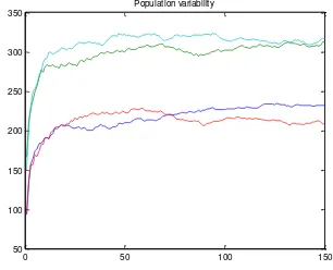
The differential evolution has a drawback, namely the continuously mutated genes can be modified in a way that they start resembling each other; in critical case the population converges into one single position. To avoid that negative feature, the training is monitored by the variances of the genes. If there are enough variations within the population, the variances of the coordinates are high. Resembling can be detected by dramatical decrease in the variance diagram. A healthy variance plot can be seen in Fig. 8.
0 50 100 150
50 100 150 200 250 300 350
Population variability
Figure 8. Variance plot to keep track on resembling
The differential evolution method is a global optimization technique, so the uniformization can be “dangerous”. If one has International Archives of the Photogrammetry, Remote Sensing and Spatial Information Sciences, Volume XXXIX-B3, 2012
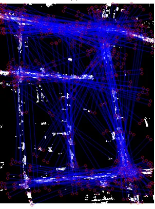
produced the final population by DE in the studied image, a strong gene multiplication can be diagnosed as in Fig. 9. A skilled human operator can extract the right candidates from the resulting set, passing them into the last phase.
Final population
Figure 9. Final population from differential evolution
The last experiment is a comparison with the artificial images to obtain recognition features of the technique. The synthetic images were processed by the same DE settings and the result is self-explainable (Fig. 10).
5. CONCLUSION
The proposed neural and genetic solution is based on pure optical image information. There was no additional help in the segmentation to extract the road pixels. Being able to execute this step on a highly reliable level, the next step can obtain better fitting performance. The original assumption was that the widely used modern neural techniques, like SVM and SOM can bring excellent result in road recognition. The first experiment series aimed to check this hypothesis. The results were surprising, because the hyperbox method could reach better scores in this test. The additional image based information band (like the NDVI) and the principal component analysis could increase the accuracy. Object oriented segmentation or more sophisticated road detection methodologies producing pixel-type result can replace the presented methods.
The biggest novelty is the application of the genetic algorithms in information retrieval from segmented images. The common genetic algorithm has a quite long run until a stable state can be reached, the new differential evolution technique can replace it because of its higher speed. The shown GA and DE methods have global optimization feature; the dependence from the implemented fitness function is crucial.
Longest 5 if the best 10 items of the final population
Figure 10. Synthetic segmentation image processed by DE algorithm (longest 5 of the 10 best genes)
More research must focus on the suitable local applicable fitness function, which is able to compile the pixels into road segments, but is fast and reliable at the same time. The genetic solution is almost independent from the image size and resolution, as well as from the number of road elements (segments), when enough genes are handled in the population. The experiment has proven that based on mutation this algorithm can extract such linear image elements.
The used software environment was Mathworks Matlab, which is an interpreter type environment. A great experience was with the differential evolution technique that it was suitable at full resolution to bring acceptable results. A future development by e.g. OpenCV can dramatically increase the size of the image to be processed.
6. REFERENCES
Beale, M.H., Hagan, M.T., Demuth, H.B., 2012. Neural
Network Toolbox. User’s Guide, R2012a, Matlab, The MathWorks Inc, Natick
Laky, S., 2012. Metaheuristic optimization in the geodesy, PhD thesis, Budapest, p. 115
Rottensteiner, F., Baillard, C., Sohn, G., Gerke, M., 2011. ISPRS Test Project on Urban Classification and 3D Building Reconstruction, ISPRS - Commission III – Photogrammetric Computer Vision and Image Analysis, Working Group III / 4 - Complex Scene Analysis and 3D Reconstruction. http://www.commission3.isprs.org/wg4/
7. ACKNOWLEDGEMENT
This work is connected to the scientific program of the "Development of quality-oriented and harmonized R+D+I strategy and functional model at BME" project. This project is supported by the New Hungary Development Plan (Project ID:
TÁMOP-4.2.1/B-09/1/KMR-2010-0002)