A SOLUTION TO LOW RFM FITTING PRECISION OF PLANETARY ORBITER
IMAGES CAUSED BY EXPOSURE TIME CHANGING
B. Liu, B. Xu, K. Di *, M. Jia
State Key Laboratory of Remote Sensing Science, Institute of Remote Sensing and Digital Earth, Chinese Academy of Sciences - (liubin, dikc, xubin, jiamn)@radi.ac.cn
Commission IV, WG IV/8
KEY WORDS: Rational Function Model, Planetary orbiter images, Sensor correction, Exposure time change
ABSTRACT:
In this paper, we propose a new solution to the low RFM fitting precision caused by exposure time changing using sensor correction. First, we establish a new rigorous geometric model, with the same ephemerides, attitudes and sensor design parameters of Chang’E-2 and HRSC images, using an equal exposure time of each scan line. The original rigorous geometric model is also established. With a given height, we can establish the correspondence between the two rigorous models. Then we generate a sensor corrected image by resampling the original image using an average elevation or a digital elevation model. We found that the sensor corrected images can be used for topographic mapping which maintains almost the same precision of the original images under certain conditions. And RFM can fit rigorous geometric model of the sensor corrected image very well. Preliminary experimental results show that the RMS residual error of the RFM fitting can reach to 1/100 pixel level too. Using the proposed solution, sensors with changing exposure time can be precisely modelled by the generic RFM.
* Corresponding author
1. INTRODUCTION
Geometric model of the sensor imagery is the basis of high accuracy geometric processing, such as topographic mapping, geometric rectification, and co-registration (Kirk et al.,2012, Toutin et al., 2004, Scholten et al.,2011). So far, most study of extra-terrestrial mapping (such as lunar and Mars mapping) uses the rigorous physical sensor model based on the collinearity equations (Di et al., 2014, Radhadevi et al., 2011, Tran et al., 2010). In order to establish the rigorous sensor model, physical parameters of the imaging sensor including ephemerides, attitudes and sensor design parameters are needed. So the rigorous physical sensor model is usually complex for scientists who are not specialized in photogrammetry. Moreover, because different orbital sensors have different geometric characteristics, the physical sensor models always differ from each other. As a result, a new corresponding physical sensor model should be developed whenever a new sensor is launched. It is challenging to implement rigorous sensors in digital photogrammetric workstations for all the orbital sensors.
In order to overcome the aforementioned disadvantages, finding a generalized geometric model which is independent of sensors and mathematically simple, to replace the rigorous physical sensor model is very meaningful. Rational Function Model (RFM) is one of the generic geometric models that have been widely used in geometric processing of high-resolution earth-observation satellite images (Tao et al., 2002, Di et al.,2003), especially when the rigorous physical sensor models are not supplied and internal geometric parameters are not disclosed. RFM consists of two cubic polynomials with 78 rational polynomial coefficients (RPCs) that can express the geometric relationship between a ground point and its corresponding image point. The model has the advantage of generality and excellent capability of fitting complex rigorous sensor models. The RPCs of the RFM can be solved under terrain-independent
and terrain-dependent computation scenarios which distinguish whether the control points generated from rigorous physical sensor model or other source (reference map etc.). A systematic investigation on the feasibility and precision of RFMs for Lunar and Mars arbiter images has been presented in our previous publications (Liu et al, 2011, Liu et al.,2014). We have established the rigorous physical sensor models of some mainstream extra-terrestrial orbiter images. Then the RFMs have been generated using terrain-independent computation scenarios. We found that Chang’E-2 and HRSC, whose exposure time changes in different scan lines, cannot be fitted by traditional RFM with the RMS residual error being up to 9 pixels. So a time-based Rational Function Model has been proposed with which the low fitting precision of Chang’E-2 and HRSC with traditional RFM can be solved precisely. The RMS residual error of time-based RFM reduces to 1/100 pixel level.
A new solution to the low RFM fitting precision caused by exposure is proposed in this paper. Sensor corrected (Liu et al., 2010) images are produced to geoprocessing instead of original images. We found that RFM can fit the sensor corrected images which product by the method proposed in this paper very well. The sensor corrected images can be used for topographic mapping which maintains almost the same precision of the original images under certain conditions.
2. METHODOLOGY 2.1 Rigorous sensor model (RSM)
The terrain-dependent computational scenarios to generate the RPCs need lots of GCPs which is hard to obtain in planetary surface. Moreover, the RFM solution is sensitive to the distribution and the number of GCPs (Tao et al., 2001). . In this paper, we focus on the study of terrain-independent The International Archives of the Photogrammetry, Remote Sensing and Spatial Information Sciences, Volume XLI-B4, 2016
computational scenarios with the physical sensor model available.
The establishment of imaging geometric model is the basis of photogrammetric stereotaxic processing, which reflects the relationship between 2D image coordinates and their corresponding 3D ground coordinates. Rigorous model describes the imaging process in the case of known sensor information, thus it is closely related to the physical and geometric characteristics of the sensors. Rigorous geometric modeling consists of exterior orientation and interior orientation and coordinate calculation based on collinearity equation. In this section, a general description of pushbroom optical rigorous physic model is given below.
2.1.1 Interior Orientation
Interior orientation refers to the transformation from image coordinates (lines and samples) to their focal plane coordinates centered at the principal point of the image. Given the focal length f of the camera and the pointing angle (X, Y) of a pixel (r, c), the focal plane coordinates of this pixel can be calculated by the interior orientation formula as follows:
tan( )
Image space coordinate system is defined using the perspective center S as its origin. X- and Y-axis are coincident with the X- and Y- axis of focal plane coordinate system, Z axis is coincident with principal optic axis, forming a right-handed coordinate system. Thus, the pointing vector u of the pixel in image space coordinate system can be presented as:
tan( )
Exterior orientation refers to the coordinate transformation from image space coordinate system to an object space coordinate system. Exterior orientation process can be expressed as:
' perspective center position in planetary body-fixed coordinate system (PBCS), respectively; Rib is the rotation matrix from image space coordinate system (ISCS) to the spacecraft body coordinate system (BCS); Rbo is the rotation matrix from BCS to orbit coordinate system (OCS); Rol is the rotation matrix from the OCS to to PBCS; ' is a scale factor; R represents the
overall rotation matrix from ISCS to PBCS. Usually, the transformation relationship between coordinate systems is determined by three Euler angles (φ, ω, ), the attitude angles (φ, ω, ) and the perspective center position (Xs, Ys, Zs) are called exterior orientation parameters (EOPs).
For push-broom CCD sensors, EOPs are changing all the time; in other words, each imaging moment has a set of EOPs. Considering the stability of the motion platform, change of
EOPs over short trajectories can be modeled using polynomials. A third-order polynomial model with imaging time as the independent variable is usually used for fitting of EOPs.
2 3 photogrammetry, which is widely used in space intersection, back projection and so on. It is established based on the principle that the perspective center, an image point and the corresponding ground point lie in a straight line. The matrix form is expressed in Eq.(3). With the collinearity equation, we can calculate the 3D ground coordinates from image coordinates with elevation or calculate the image coordinates from 3D ground coordinates.
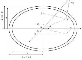
Planets can be considered as an ellipsoid which is formed by rotation around its rotational axis. We define the equatorial radius of a planet is a and the polar radius is b; assuming that a ray from the perspective center S(Xs, Ys, Zs) intersects the planet at a ground point M(XM,YM,ZM) which has an elevation of h (See Fig.1),
Figure 1. Ground point calculation by space
It can be deduced according to Eq.(3):
1
Eq.(3). Eq.(6) can be further written as Eq.(7).
1 The International Archives of the Photogrammetry, Remote Sensing and Spatial Information Sciences, Volume XLI-B4, 2016
Considering that the ray actually intersects an ellipsoid with three semi-principal axes of length a+h, a+h, b+h, thus, it can be also deduced as follows:
Hence, the two roots of the equation are:
2 range or which has the relative short distance from perspective center S to the two intersection points, the fake solution can be eliminated and the correct solution is kept.
Back projection refers to the transformation from a ground point to its corresponding image point. For push-broom CCD sensor, back projection can be performed using binary searching method. Given the ground coordinates, the image coordinates are calculated with EOPs of the middle scan line using Eq.(5); by comparing the calculated x value to the theoretical x value (row direction), focal plane coordinates continue to be calculated using the upper or lower half of EOPs until the difference between the calculated value and theoretical value is less than a pre-defined threshold. The EOPs which can get the closest x value are finally chosen to calculate the image coordinates of this point (see Fig.2).
Ground coordinates Exterior orientation parameters
Is the difference between x and theoretical value less
than the threshold Taking EOPs of the middle scan line
Calculating focal plane coordinates(x, y)
Calculating (x, y) with EOPs in a window centered at this scan line
Taking the EOPs which get the closest x value as the true EOPs of this point
Figure 2. Back projection using binary searching
2.2 Construction of rational function model
Rational function model (RFM) is a commonly used generic geometric model. It is a mathematical fitting of rigorous geometric model, and has many advantages of platform independence, simple form, and high calculation speed. It has been widely used in photogrammetric processing of high-resolution earth observation images.
2.2.1 Rational function model
The RFM can be used to establish the relationship between image-space coordinates and object-space coordinates with the ratios of polynomials (Di et al., 2003), as shown in Eq. (11):
1 function Pi, named as the rational polynomial coefficients (RPCs).
2.2.2 Solution of rational polynomial coefficients
Construction of a RFM is actually the process of fitting the rigorous geometric model with RFM and solving RPCs. It can be divided into two steps: virtual control points generation and RFM solution.
First, grid points are generated in image space with a certain interval in x and y directions. Then the elevation is sliced into several layers in object space, and the corresponding ground points are generated using the rigorous sensor model. These image points and ground points are called virtual control points and used for fitting rigorous model with RFM. Finally, the RPCs are derived by these virtual control points through least squares fitting.
2.2.3 Coordinate calculation using RFM
Once the RPCs of a sensor model are solved, we can easily realize space intersection and back projection using RFM. Given a ground point (P, L, H), the corresponding image point (x, y) is solved directly by Eq.(11).
Inversely, given at least two conjugate image points, observation equations can be derived after linearization:
11 12 13
And the ground point can be solved using least-squares method. Compared with the solution process using rigorous geometric model, RFM is a simpler way to describe the imaging process and spatial relationship.
2.3 Time-based rational function model
When traditional RFM is used to fit CE-2 CCD and HRSC imagery, fitting results cannot reach a high precision, even though image size is quite small. The solution is easily ill-posed and the RPCs are usually abnormal values.
Through a lot of analysis and experiments, we found that this kind of situation is caused by integration time hop of CE-2 CCD camera. The design of time delayed integration (TDI) for CE-2 CCD camera ensures the imaging clear in different orbit altitudes. When orbit altitude changes, integration time hops to keep a certain velocity-height ratio. For this reason, there is no longer a linear relationship between the image scan time and the image coordinate r, and the traditional RFM is not applicable for CE-2 CCD imagery. Thus, we propose a time-based RFM to fit the rigorous geometric model of CE-2 CCD imagery.
Time-based RFM is established by fitting image scan time t instead of image coordinate r, it can be expressed as Eq. (14).
1 regularization parameters of scan time t.
The solution process of time-based RFM can be divided into three steps:
(1) Constructing the relationship between image coordinate (rn, cn) and ground coordinate (Xn, Yn, Zn) to generate the virtual control point grid
(2) Establishing a piecewise function tn = f1(rn) to describe the relationship between tn and rn, so that rn can be transformed to tn by piecewise linear interpolation.
(3) RPCs of the time-based RFM can be solved, and the scan time-scan line index table is recorded along with the RPCs together.
2.4 Sensor Corrected (SC) image resample
As the satellite orbital altitude changes during operation, the pushbroom imaging satellite’s integration time of a line also has a corresponding transition. To obtain optimum width and image quality, high-resolution satellites were powered by a multi-CCD mosaic approach (Liu et al., 2010). Due to technical and physical characteristics of CCD constraints, the CCD cannot be a straight line in the focal plane. In this paper, a virtual linear array CCD is proposed to solve the low fitting precision caused
by integration time changing and stitch the images of multi-CCDs.
2.4.1 Virtual CCD linear array
The virtual CCD linear array is continuous, linear, and parallel. It has the same number of cross-track samples as the original CCD array. A virtual pushbroom camera is built to reconstruct the originally obtained image. A more complete description of the virtual camera, along with the image characteristics required to support this model, is provided below.
Optical distortion removed.
Focal Plane Assembly consisting of one continuous, perfectly linear detector.
The focal length of the camera model will be the same as the effective focal length of the original camera model.
A single image row represents one virtual time which has the same integration time.
2.4.2 Resampling of SC images
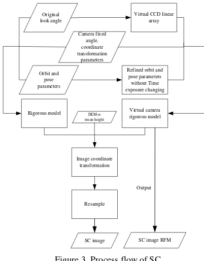
After calibration of the camera, interior parameters of the camera can be expressed as each CCD point angle (X, Y). According to the original camera parameters, a virtual linear array CCD is established. With interior orientation elements and exterior orientation elements obtained, the rigorous geometric model of original and SC images can be built according to the Collinearity Equation. The relationship between the coordinates of the SC image and the original image is established using the data provided by DEM or a given mean height of the image area. With the pixel coordinates corresponding relationship, the SC image can be resampled.
Original
Figure 3. Process flow of SC
Using the RSM of SC image, we can establish the RFM of SC image. For the SC image integration time was refined, the RFM fitting precision will be high.
3. EXPERIMENTAL RESULTS AND DISCUSSIONS 3.1 Data set
In order to perform a systematic investigation of RFM fitting the physical sensor model capability in planetary mapping area. Some mainstream planetary obiter imagery, which including Lunar obiter and Mars orbiter, such as Lunar Reconnaissance Orbiter Camera (LROC) ( Robinson et al.,2010, Vondrak et al., 2010) Narrow Angle Camera (NAC), Chang’E-1 (CE-1), Chang’E-2 (CE-2), high-resolution stereo camera (HRSC) on Mars Express (Jaumann et al., 2007), and Mars Reconnaissance Orbiter’s High Resolution Imaging Science Experiment (HiRISE) ( McEwen et al.,2007) are used in the experiment. LRO NACs consists of two identical monochrome push-broom scanner, which can acquire high resolution images of Lunar surface with a pixel scale of 0.5m (which is the highest resolution of Lunar orbiter imagery) from a 50km orbit. China’s CE-1 and CE-2 cameras are similar in design have the ability to obtain near-simultaneous imaging data with along-track stereo. The resolution gap between the two cameras is huge, from 120m of Chang’E-1 to 7m of ChangE’2. And 1.5m resolution images at the perilune on 100*15 km elliptical orbit were also acquired at the CE-3 landing site—Mare Imbrium and Sinus Iridum (mostly but not completely covered) by CE-2. The HiRISE experiment of MRO is characterized by high SNR and has a maximum spatial resolution of 0.3 m/pixel, which can generate the most detailed DTM with 1m /pixel. The HRSC (Jaumann et al., 2007) is the only dedicated stereo camera orbiting Mars with nine CCD line detectors mounted in parallel on a focal plane. The HRSC spatial resolution is 10 m/pixel at the nominal periapsis altitude of 250km. The HiRISE and HRSC contains very the high-resolution and the high- to
medium-resolution images of Mars which are essential in detailed surface exploration.
The orbit (Nos. 0562 with 120m/pixel) of CE-1 image located at Sinus Iridum and Tow orbits (Nos.0570 with 7m/pixel, Nos.0236 with 1.5m/pixel) located at Mare Imbrium which covers the landing site of Chang'E-3(CE-3) lunar rover are used in our experiments. The LRO NAC image M1154358210RE (0.25 m/pixel) which also locate in CE-3 site used in the experiment too. Two HiRISE cross track stereo images (ESP_028256_9022_RED3_0, ESP_028269_1755_RED3_0) and HRSC along track stereo images (H4235_0001_S12, H4235_0001_S2) were also chosen as experimental data.
The images used in this experiment include Lunar and Mars image of different orbiters at different resolutions (from very high to medium).
3.2 RFM fitting precision
The RSMs of above orbiter images are established and the terrain-independent scenario is used to fit their RFMs. The fitting errors of CE-1, LRO NAC and HiRISE, shown in Table 1, are all at sub-pixel level, which can be ignored for subsequent mapping with the consideration of the precision of image matching in geopositioning. The fitting errors of CE-2 and HRSC in line direction are relatively high while the precisions in row direction are not good enough, which can reach approximately 10 pixels, and the RFM solving process is not stable. These fitting errors will have severe influence on subsequent mapping process.
Table 1. Residuals of traditional RFM fitting of different planetary orbiter images
3.3 Time based RFM fitting precision
The low fitting precision of CE-2 and HRSC images is caused by integration time changing.
T = 2.85ms+N*13.92us (16)
Eq. (16) is used to calculate the integration time of CE-2, from which it can be seen that the change of row integration time with N is not continual. Figure 4 is part of the row integration
time change of CE-2 and figure 5 is the enlarged view of the red rectangle in figure 4.
Data length
(pixel)
width (pixel)
Resolution (m/pixel)
RMSE (row)
(pixel)
RMSE (column)
(pixel)
RMSE (pixel)
LRO NAC 52224 5064 0.5 0.02 0.09 0.09
CE-1 10000 512 120 0.02 0.01 0.02
CE-2
200000 6144 7 0.04 8.01 8.01
100000 6144 7 0.00 7.87 7.87
50000 6144 1.5 0.00 94.30 94.30
3000 6144 1.5 0.00 5.19 5.19
HiRISE ESP_028256_9022_RED3_0 85000 1024 0.25 0.13 0.05 0.14
ESP_028269_1755_RED3_0 115000 1024 0.25 0.00 0.00 0.00
HRSC h4235_0001_s12 16784 5176 17.2 0.00 9.26 9.26
h4235_0001_s22 15824 5176 15.6 0.00 9.79 9.79
Figure 4. The change of integration time of CE-2
Figure 5. Enlarged view of the red rectangle in Figure 4
Similarly, the row integration time of HRSC cameras also change with the variation of orbiter height. Figure 6 and Figure 7 are row integration time of h4235_0001_s12 and h4235_0001_s22, respectively.
Figure 6. Integration time of h4235_0001_s12
Figure 7. Integration time of h4235_0001_s22
In order to tackle the problem of poor fitting precision caused by row integration time change, this paper presents the time-based RFM and applies it to process CE-2 and HRSC images. The fitting residuals of the time-based RFM are demonstrated in Table 2. It can be concluded that the time-based RFM can effectively solve the pool precision problem produced by traditional RFM.
Data
Traditional RFM(pixel)
Time-based RFM(pixel) RMSE
(column)
RMSE (row)
RMSE (column)
RMSE (row) 200,000 lines
CE-2 0.04 8.01 0.04 0.00
100,000 lines 0.00 7.87 0.00 0.00
50,000 lines 0.00 94.30 0.00 0.00
30,000 lines 0.00 5.19 0.00 0.00
h4235_0001_s1
2 0.00 9.26 0.00 0.00
h4235_0001_s2
2 0.00 9.79 0.00 0.00
Table 2. Fitting residuals of time-based RFM
3.4 SC image processing
The method described above is applied to HRSC stereo images and the RFMs of the SC images are fitted. The virtual re-imaged SC images do not contain integration time change, so the fitting precision of SC RFM of images can satisfy the requirement of high-precision mapping. The fitted residuals of time-based RFM are displayed in Table 3.
Data
Original images RFM(pixel)
SC images RFM(pixel) RMSE
(column)
RMSE (row)
RMSE (column)
RMSE (row)
h4235_0001_s12 0.00 9.26 0.00 0.00
h4235_0001_s22 0.00 9.79 0.00 0.00
Table 3. Fitting residuals of original and SC images RFM
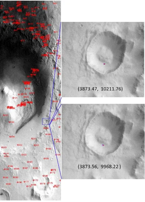
Figure 8. The distribution of corresponding points in HRSC stereo images (left); A corresponding point pair in h4235_0001_s12 original image (upper-right) and resampled image (lower-right)
The corresponding points in original stereo images and resampled SC stereo images are located respectively. Figure 8 shows that the difference of row coordinates between original and SC images are up to 200 pixels.
The ground coordinates generated from forward intersections based on the RSM of original images and the RFM of SC
Table 4. The coordinate differences generated from forward intersections based on the RSM of original images and the RFM of SC images
It can be seen that the differences between two results are 1.33 m in total. Considering that the image resolution is about 15 m, the residuals of SC image RFM can be ignored and the SC images can replace original images to realize high-precision geopositioning and mapping.
4. CONCLUSIONS
A systematic investigation on the feasibility and precision of RFMs for Lunar and Mars arbiter images has been presented in this paper. Time-based RFM and sensor corrected images RFM were proposed to solve the low fitting precision caused by exposure time changing in some orbiters, such as CE-2 and HRSC. According to our experiments with HRSC stereo images, we found the SC images can replace original images to realize high-precision geopositioning and mapping. More study will be performed on using this method to stitch the multiple CCD images in one sensor such as HiRISE.
ACKNOWLEDGMENTS
This study was supported in part by National Key Basic Research and Development Program of China under Grant 2012CB719902 and in part by National Natural Science Foundation of China under Grant 41590851 and 41301528. We would like to thank the LROC, HRSC, HiRISE team for making the LROC NAC, HRSC and HiRISE images available online. We also would like to thank the Lunar and Deep Space Exploration Science Applications Center of the National Astronomical Observatories (NAOC) and Beijing Aerospace Control Center for providing the CE-2 images and telemetry data respectively.
REFERENCES
Di, K., Y. Liu, B. Liu, M. Peng and W. Hu, 2014. A Self-calibration bundle adjustment method for photogrammetric processing of Chang'E-2 stereo lunar imagery. IEEE Transaction on Geoscience and Remote Sensing, 52(9), pp.5432-5442.
Di, K., R. Ma, and R. Li, 2003. Rational Functions and Potential for Rigorous Sensor Model Recovery. Photogrammetric Engineering and Remote Sensing, 69(1), pp. 33-41.
Jaumann, R., G. Neukum, T. Behnke, T. Duxbury, K. Eichentopf, J. Flohrer, et al., 2007. The high-resolution stereo camera (HRSC) experiment on Mars Express: Instrument aspects and experiment conduct from interplanetary cruise through the nominal mission. Planetary and Space Science, 55, pp. 928-952.
Kirk, R., B. Archinal, L. Gaddis and M. Rosiek, 2012. Lunar Cartography: Progress In The 2000s and Prospects for the 2010s. In: International Archives of the Photogrammery, Remote sensing and Spatial Information Sciences, B4, pp. 489-494.
Liu, B., G. Zhang, H. B. Pan and W.S. Jiang, 2010. Production and characteristics of Sensor Corrected and geooded ellipsoid corrected products. In: Informatics and Computing (PIC), Shanghai, China, IEEE International Conference on.
Liu, B., Y. Liu, K. Di and X. Sun, 2014. Block adjustment of Chang'E-1 images based on rational function model. In: Remote Sensing of the Environment: 18th National Symposium on Remote Sensing of China, International Society for Optics and Photonics, pp. 91580G-91580G.
Liu, Y. and K. Di, 2011. Evaluation of Rational Function Model for Geometric Modeling of Chang’E-1 CCD Images. In: International Achieves of the Photogrammetry, Remote Sensing and Spatial Information Sciences, Guilin, China, Vol. 38, Part 4/W25, pp. 121-125.
McEwen, A., E. Eliason, J. Bergstrom, N. Bridges, C. Hansen, W. Delamere, et al., 2007. Mars reconnaissance orbiter's high resolution imaging science experiment (HiRISE). Journal of Geophysical Research: Planets (1991–2012), 112, E05S02.
Radhadevi, P., V. Nagasubramanian, S. Solanki, T. Sumanth, J. Saibaba and G. Varadan, 2011. Rigorous Photogrammetric Processing of Chandrayaan-1 Terrain Mapping Camera (TMC) Images for Lunar Topographic Mapping. In: Lunar and Planetary Science Conference, Texas, USA, 42, pp. 1384.
Robinson, M., S. Brylow, M. Tschimmel, D. Humm, S. Lawrence, P. Thomas, B. Denevi, E. Bowmancisneros, J. Zerr, M. Ravine, M. Caplinger, F. Ghaemi, J. Schaffner, M. Malin, P. Mahanti, A. Bartels, J. Anderson, T. Tran, E. Eliason, A. Mcewen, E. Turtle, B. Jolliff and H. Hiesinger, 2010. Lunar Reconnaissance Orbiter Camera (LROC) instrument overview. Space Science Reviews, 150, pp. 81-124.
Scholten, F., J. Oberst, K. Matz, T. Roatsch, M. Wahlisch, P. Glaser, M. Robinson, E. Mazarico, G. Neumann, M. Zuber and D. Smith, 2011. Complementary LRO Global Lunar Topography Datasets — A Comparison of 100 Meter Raster DTMs from LROC WAC Stereo (GLD100) and LOLA Altimetry Data. In: Lunar and Planetary Science Conference, Texas, USA, 42, pp. 2080.
Tao, C. and Y. Hu, 2001. A comprehensive study of the rational function model for photogrammetric processing. Photogrammetric Engineering and Remote Sensing, 67, pp. 1347-1357.
Tao, C. and Y. Hu, 2002. 3D reconstruction methods based on the rational function model. Photogrammetric Engineering and Remote Sensing, 68, pp. 705-714.
Toutin, T., 2004. Review article: Geometric processing of remote sensing images: models, algorithms and methods. International Journal of Remote Sensing, 25, pp. 1893-1924.
Tran, T., E. Howingtonkraus, B. Archinal, M. Rosiek, S. Lawrence, H. Gengl, D. Nelson, M. Robinson, R. Beyer, R. Li, J. Oberst and S. Mattson, 2010. Generating Digital Terrain Models from LROC Stereo Images with SOCET SET. In: Lunar and Planetary Science Conference, Texas, USA, 41, pp. 2515.
Vondrak, R., J. Keller, G. Chin, and J. Garvin, 2010. Lunar Reconnaissance Orbiter (LRO): Observations for lunar exploration and science. Space science reviews, 150, pp. 7-22.