Directory UMM :Data Elmu:jurnal:E:Energy Economics:Vol22.Issue3.2000:

(1)

Estimation of international output

]

energy

relation: effects of alternative output

measures

Ram M. Shrestha

U

Energy Program, School of En¨ironment, Resources and De¨elopment, Asian Institute of Technology, P.O. Box 4, Klong Luang, Pathumthani 12120, Thailand

Abstract

This paper analyzes the output]energy relationship with alternative measures of output and energy. Our analysis rejects the hypothesis of non-diminishing returns to energy consumption when GDP at purchasing power parities is used as the output measure unlike the case with GNP at market exchange rates. This finding also holds when energy input includes the usage of both commercial and traditional fuels.Q_{2000 Elsevier Science B.V.}

JEL classifications:C52; Q43

Keywords:Output]energy relation; GDP at market exchange rates; GDP at purchasing power parity; Output returns to energy

1. Introduction

The issue of output and energy relation, in particular, whether there exist diminishing returns to energy use, has received attention in some recent energy

Ž .

economics literature. In two interesting papers, Moroney 1989 and Moroney et al.

Ž₁₉₉₀. Ž_{hereafter ‘MSV’ have analyzed the relationship between GNP per capita}.

Ž .

and energy consumption per capita. Moroney 1989 stated that the ‘...wealthiest

U

Fax:q66-2-5245439.

Ž .

E-mail address:ram@ait.ac.th R.M. Shrestha

Ž .

(2)

( ) R.M. ShrestharEnergy Economics 22 2000 297]308

298

countries exhibit a sharply diminishing real income response with respect to higher

Ž . Ž

energy use’ p. 3 . However, MSV, using a smaller but more credible data set they

.

omitted countries with obviously questionable data , found evidence of non-di-minishing returns to energy per capita. The finding of non-dinon-di-minishing output returns to energy is counterintuitive as it implies that output could grow with energy input at a non-decreasing rate with all other factors remaining unchanged.

Ž .

Moroney 1989 and MSV also analyzed the appropriateness of selected functional

Ž

forms to characterize the relationship between output and energy MSV con-sidered three specific functional forms, i.e. linear, semi-log and double-log while

Ž . .

Moroney 1989 also considered the semi-log quadratic function . Statistical tests in

Ž .

both Moroney 1989 and MSV selected the double-log functional form for

characterizing the output]energy relationship.

Ž .

Both Moroney 1989 and MSV examined the output]energy relationship through

Ž .

a model with single input i.e. energy . They used, as the measure of output, GNP

Ž .

calculated at market exchange rates GNP_{ME R} not GDP at purchasing power

Ž .

parities GDP_{PP P} . GDP_PPP is particularly attractive in that it gives a more accurate

representation of the output for economies that do not have a free market for

Ž .

foreign currency exchange. Although Moroney 1989 expressed the desirability of

using GDP_{PP P}, he also stated: ‘I doubt these alternati¨e measures of real output would

Ž .

make much difference in the statistical results.’ Footnote 10, p. 8 . However, as there

is no fixed and uniform ratio for converting GNP_{ME R}to GDP_PPP across countries,

that statistical results on the relationship are invariant with respect to the type of output measure used is a hypothesis to be tested rather than a plausible

assump-tion. It could also be argued that the use of GDP_{ME R} as an output measure is

preferable to that of GNP_{ME R} on the grounds of data consistency since available

data on energy consumption are limited to domestic energy consumption and thus

the use of GNP_{ME R} to represent output and domestic energy consumption as the

input would give a distorted picture of the energy intensity of a country’s output.

Ž .

Furthermore, Moroney 1989 and MSV used only commercial energy consumption

Ž

as the measure of energy input and ignored the use of traditional fuels e.g.

.

fuelwood, and agricultural residues . Given the relatively heavy dependence of developing countries on traditional fuels, the exclusion of these fuels is likely to

introduce an error in the estimation of the output]energy relationship. It is

therefore of interest to examine whether the output]energy relation is

substan-tially affected by an exclusion of traditional fuels from the energy consumption data.

This study examines the effects on output]energy relationship of using

alterna-tive measures of output, i.e. GDP_{ME R} and GDP_PPP as the output measure as

compared to the case in which GNP_{ME R} is used. It also analyzes the effects of the

inclusion of traditional fuels in energy consumption. It uses a more recent cross sectional data set of 41 countries in 1988, 1989, and 1990 than MSV who used data of 1978, 1979 and 1980.

(3)

returns to energy use per capita is rejected when GDPPP P is used as the output

measure while it is accepted when GNPME R is used as the output measure. This

result remains valid regardless of whether traditional fuels were included in energy consumption.

2. The model

Denoting Y for GNP per capita and X for energy consumption per capita, we

estimate the parameters of the following three models relating output with energy consumption as in MSV:

Ž .

Linear: YsaqbX 1

aqbX _{Ž .}

Semi-logarithmic: Yse 2

b _{Ž .}

Double-logarithmic: YsAX 3

As MSV observe, the linear model permits neither increasing nor decreasing

Ž 2 2 _.

returns to energy per capita sinceY0'd YrdX s0 while the semi-logarithmic

Ž 2 _.

model allows only increasing returns since Y0sb Y)0 . Unlike the linear and

semi-log models, the double-log model allows either increasing, constant, or

Ž

decreasing returns to energy per capita as b), s, or -1 since Y0 sb by

. by2

1 AX .

Also as in MSV, we estimate the following general Box]Cox model:

Žl1. Žl2. Ž .

Note here that the linear, semi-log and double-log models in Eqs. 1 ]3 ,

respec-Ž .

tively i.e. the ‘restricted’ models are the special cases of the Box]Cox model: i.e.

linear, if l₁sl₂s1; semi-log, if l₁s0,l₂s1; and double-log, if l₁sl₂s0.

Ž . Ž

The parameters of the Box]Cox general model in Eq. 4 i.e. the ‘unrestricted’

.

model was estimated by the maximum likelihood method using the software TSP

ŽVersion 4.3 see Hall 1996 . As in MSV, the test statistic for testing whether a.w Ž .x

restricted model best represents the relationship between the real output per

capita and energy per capita is x2 distributed with 2 d.f. and is expressed as:

w Ž . Ž . x 2 _{Ž .}

(4)

300

Ž . Ž .

where, L l1,l2 UR and L l1,l2 R are the maximum likelihood ratio values of the

unrestricted and restricted models, respectively.

3. Data and their sources

Cross-sectional data from 1988 to 1990 for 41 countries were used in the

estimation of output]energy relationship with GNPME R and GDPPPP as output

measures while the data set involving GDPME R was smaller and involved 31

countries only as GDPME R data for some countries were obviously questionable

and were therefore excluded. The countries included in this study are listed in Appendix A.

Data on GNP_{ME R} per capita and GDP_PPP per capita were obtained from UNDP

Ž1991, 1992, 1993 while data on GDP. _{ME R}were taken from IMF 1993 . The sourceŽ .

Ž

for per capita commercial energy consumption data was World Bank 1990, 1991,

.

1992 . Traditional energy consumption data for 1989 were obtained from WRI

Ž1992 ..

4. Results

4.1. Effects of using alternati¨e output measures

Ž

Tables 1]3 present the maximum likelihood estimates of parameters a,b,l₁,

.

l₂ of the generalized Box]Cox model along with the ordinary least squares

estimates of parameters a andb of double-log, semi-log and linear models when

the output is measured by GNP_{ME R}, GDP_MER and GDP_PPP, respectively. The

tables also show the associated values of R2_{, the maximum of log likelihood}

w Ž .x 2 _w

function i.e. L l₁,l₂ and the calculated values of x test statistic as defined in

Ž .x 2

Eq. 5 . Note that R values across the models here are not directly comparable as

the dependent variables are not the same for each model. Following Kennedy

Ž_{1992, p. 102 and Gujarati 1995, pp. 209}. Ž _]_{210 , we have also calculated}. _R2 _values

Ž . Ž .

for Models 1 and 4 in a manner that makes them comparable to the values

Ž . Ž .1

calculated by Models 2 and 3 . These are also presented in the tables.

As can be seen from the tables, of the three restricted models considered, the

calculated values of x2 statistic in the case of the double-log model were less than

Ž .

the critical value at the 5% significance level i.e. 5.991 for sample data of each of

Ž . 2

the 3 years considered i.e. 1988, 1989, and 1990 . However, the calculated x

values were greater than the critical values at both 5% and 1% levels for both linear and semi-log models. Thus, the double-log model could not be rejected

1

The following procedure was used in the derivation of the comparable value ofR2. First, the estimated

ˆ ˆ

Ž . Ž .

values of Yi i.e.Yi from the ‘optimal’ i.e. Box]Cox and linear models are converted into lnYi. Then

2 _ˆ

(5)

Table 1

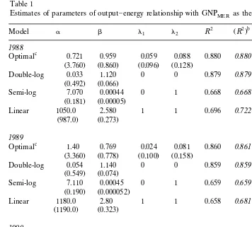
a Estimates of parameters of output]energy relationship with GNPME Ras the output measure

2 _Ž 2 b_. _Ž _. 2

Model a b l₁ l₂ R R Ll₁,l₂ x₂

1988

c

Optimal 0.721 0.959 0.059 0.088 0.880 0.880 y364.381 0

Ž3.760. Ž0.860. Ž0.096. Ž0.128.

Double-log 0.033 1.120 0 0 0.879 0.879 y364.765 0.768

Ž0.492. Ž0.066.

Semi-log 7.070 0.00044 0 1 0.668 0.668 y385.518 42.274

Ž0.181. Ž0.00005.

Linear 1050.0 2.580 1 1 0.696 0.722 y401.0 73.238

Ž987.0. Ž0.273. 1989

c

Optimal 1.40 0.769 0.024 0.081 0.860 0.861 y372.064 0

Ž3.360. Ž0.778. Ž0.100. Ž0.158.

Double-log y0.054 1.140 0 0 0.859 0.859 y372.325 0.522

Ž0.549. Ž0.074.

Semi-log 7.110 0.00045 0 1 0.659 0.659 y390.395 36.662

Ž0.190. Ž0.000052.

Linear 1180.0 2.80 1 1 0.658 0.681 y408.0 71.872

Ž1190.0. Ž0.323. 1990

c

Optimal 0.903 0.901 0.041 0.081 0.858 0.858 y376.309 0

Ž3.920. Ž0.901. Ž0.104. Ž0.160.

Double-log y0.115 1.150 0 0 0.857 0.857 y376.576 0.534

Ž0.564. Ž0.075.

Semi-log 7.190 0.00045 0 1 0.651 0.651 y394.870 37.122

Ž0.194. Ž0.000053.

Linear 1360.0 3.030 1 1 0.651 0.662 y412.0 71.382

Ž1300.0. Ž0.355.

a

Figures inside parentheses represent standard errors of the estimated parameters. b

These figures represent the values of R2 that are comparable to those of double and semi-log

Ž .

models i.e. with logYas the dependent variable . c

‘Optimal’ here refers to the Box]Cox model.

irrespective of the output measures considered while both the linear and semi-log models were rejected.

Ž .

The estimated coefficient of energy consumption per capita i.e. b for the

double-log model with GNP_{ME R} as the output measure was found to range from

Ž .

1.12 to 1.15 all statistically significant at 5% . Note that the estimated values of b

Ž .

in Table 1 are higher than those reported by MSV i.e. 0.890]0.914 . The values of

b with GDP_{ME R} as the output measure varied from 0.925 to 0.934 while those in

the case of GDP_pppwere in the range 0.614]0.658.

The hypothesis of non-diminishing returns to energy per capita was not rejected

at the 5% significance level for all 3 years in the GNP_{ME R} case as in MSV. In the

(6)

302 Table 2

a Estimates of parameters of output]energy relationship with GDPME R as the output measure

2 _Ž 2 b_. _Ž _. 2

1988

c

Optimal y1.050 1.700 0.123 0.055 0.950 0.950 y258.463 0

Ž5.190. Ž1.290. Ž0.128. Ž0.129.

Double-log 1.320 0.934 0 0 0.951 0.951 y259.244 1.562

Ž0.297. Ž0.039.

Semi-log 7.120 0.00038 0 1 0.714 0.714 y286.597 56.268

Ž0.180. Ž0.000044.

Linear 1030.0 1.830 1 1 0.853 0.869 y280.0 43.074

Ž575.0. Ž0.141. 1989

c

Optimal 0.097 1.380 0.081 0.034 0.937 0.939 y263.039 0

Ž4.450. Ž1.230. Ž0.132. Ž0.148.

Double-log 1.370 0.925 0 0 0.939 0.939 y263.340 0.602

Ž0.333. Ž0.044.

Semi-log 7.120 0.00038 0 1 0.716 0.716 y287.182 48.286

Ž0.182. Ž0.000044.

Linear 1040 1.820 1 1 0.825 0.860 y283.0 39.922

Ž646.0. Ž0.156. 1990

c

Optimal 0.013 1.400 0.084 0.036 0.933 0.935 y264.484 0

Ž4.550. Ž1.240. Ž0.122. Ž0.144.

Double-log 1.350 0.930 0 0 0.935 0.935 y264.793 0.618

Ž0.347. Ž0.046.

Semi-log 7.150 0.00037 0 1 0.706 0.706 y288.114 47.26

Ž0.184. Ž0.000044.

Linear 1130 1.82 1 1 0.810 0.847 y285.0 41.032

Ž678.0. Ž0.164.

a

Ž .

except with the data set of 1989. The hypothesis in this case was, however, rejected for all 3 years at the 10% significance level.

Interestingly, in the GDP_ppp case, the hypothesis of non-decreasing output

returns to energy per capita was consistently rejected for all 3 years even at the 1%

significance level. This is contrary to the finding of MSV in the GNP_{ME R} case.

Clearly, output returns to energy is found to be sensitive to the choice of the

output measure. Note that for the reasons stated earlier, GDP_{PP P} is considered to

be a better measure of output for cross country studies and the present analysis

shows the output returns to energy use to be diminishing when GDP_{PP P} is used as

the output measure.

(7)

Table 3

a Estimates of parameters of output]energy relationship with GDPPP P as the output measure

2 _Ž 2 b_. _Ž _. 2

1988

c

Optimal 7.140 0.766 0.133 0.130 0.897 0.896 y357.324 0

Ž4.710. Ž1.090. Ž0.209. Ž0.135.

Double-log 4.250 0.614 0 0 0.894 0.894 y358.027 1.404

Ž0.250. Ž0.034.

Semi-log 8.10 0.00025 0 1 0.703 0.703 y379.233 43.816

Ž0.093. Ž0.000026.

Linear 3140.0 1.880 1 1 0.793 0.828 y377.0 39.350

Ž554.0. Ž0.154. 1989

c

Optimal 9.560 0.749 0.185 0.197 0.893 0.891 y361.009 0

Ž7.770. Ž0.993. Ž0.2. Ž0.164.

Double-log 4.240 0.620 0 0 0.886 0.886 y362.478 2.938

Ž0.266. Ž0.036.

Semi-log 8.120 0.00025 0 1 0.723 0.723 y380.635 39.252

Ž0.092. Ž0.000025.

Linear 3090.0 2.040 1 1 0.818 0.843 y378.0 33.982

Ž566.0. Ž0.154. 1990

c

Optimal 6.260 1.380 0.190 0.130 0.865 0.861 y371.792 0

Ž7.070. Ž2.0. Ž0.226. Ž0.172.

Double-log 4.040 0.658 0 0 0.862 0.862 y372.632 1.680

Ž0.315. Ž0.042.

Semi-log 8.190 0.00026 0 1 0.665 0.665 y390.780 37.976

Ž0.108. Ž0.000029.

Linear 3690.0 2.190 1 1 0.735 0.861 y390.0 36.416

Ž775.0. Ž0.211.

a

Ž .

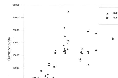
less than that in the GDP_{ME R}case. In most low income developing countries which

are at the lower range of energy consumption per capita, the reported values of

GDP_{PP P} are higher than the corresponding value of GNP_MERwhile the opposite is

the case for most high income industrialized countries which have a higher level of

Ž .

energy consumption see Fig. 1 . Similar observations can be made between

GDPPP P and GDPMER cases. This indicates that, with other things remaining the

Ž .

same, the estimated value of b with the ‘correct’ measure of output i.e. GDPPP P

would be smaller than those in cases with GNPME R and GDPMER.

4.2. Effects of inclusion of traditional energy consumption

(8)

()

R.M.

Shrestha

r

Energy

Economics

22

2000

297

]

308

304

(9)

Ž_{i.e. ‘modern’ fuels in the energy input. However, it is well-known that unlike}.

industrialized countries, developing countries have high dependence on traditional fuels. Although the data on traditional fuel consumption are far less reliable than

Ž .

the commercial energy data, especially in developing countries a study of

output]energy relationship cannot totally ignore the use of traditional fuels given

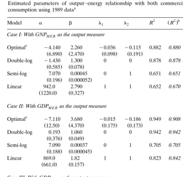
the latter’s importance in developing countries. In order to gain some insight into the order of magnitude of the effects of traditional fuel consumption, we estimated

Ž . Ž .

the parameters of Eqs. 1 ]4 with the 1989 data of 31 countries by including the

use of both commercial and traditional fuels in the input measure. The results are presented in Table 4. The log-linear model was again preferred to semi-log and

linear models. The estimated values of b in GNP_{ME R,}GDP_MER and GDP_PPP cases

are 1.300, 1.060 and 0.711, respectively. Two observations are interesting to make:

first, for each of the output measures considered, the estimated values of b are

now consistently higher than the corresponding figures when only commercial fuels were included in energy consumption. Secondly, the hypothesis of increasing output returns to energy consumption is rejected even at the 1% significance level

in the GDPPP P case while it is not rejected in both GNPMER and GDPMERcases at

the 5% significance level. In other words, with correct measures of output and energy consumption, the results of this study give a strong indication that output per capita exhibits non-increasing returns to energy consumption contrary to the findings of MSV.

4.3. Robustness of the estimated parameters

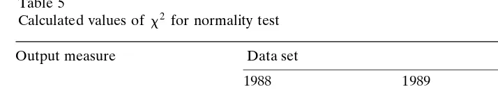
As in MSV, the stability of the estimated parameter values over the selected years in the study were examined using the Chow-test. The calculated values of

F_4,117 in the GNP_MER, GDP_MER and GDP_PPP cases are 0.2642, 0.0096 and 1.1485,

respectively, well below the critical value of 2.45 at the 5% significance level. Thus, the hypothesis that the estimated values of parameters were robust over the years could not be rejected in any of the cases considered. As normality of residuals is

w

assumed in the Chow-test, it was examined through the Jarque]Bera test see e.g.

Ž . x Ž

Kmenta 1986 , pp. 265]267 . The values of the test statistic for this purpose which

2 _.

is x2 distributed for the data sets of 1988, 1989 and 1990 for each type of output

measure and commercial energy consumption are presented in Table 5. Note that

2 _Ž 2

the calculated values of x2 are all -5.991 i.e. the critical value of x2 at the 5%

.

significance level . Thus, the hypothesis of the normality of residuals could not be rejected for any of the data sets.

5. Conclusions and final remarks

The estimated values of coefficients of energy consumption per capita in the

GDP_{PP P} case were found to be consistently below one and smaller than that in the

GNP_{ME R} and GDP_MER cases. Inclusion of traditional fuels in energy consumption

(10)

306 Table 4

Estimated parameters of output]energy relationship with both commercial and traditional energy a

consumption using 1989 data

2 _Ž 2 b_. _Ž _. 2

Case I: With GNP_{M E R}as the output measure

c

Optimal y4.140 2.260 y0.036 y0.115 0.882 0.880 y368.835 0

Ž6.890. Ž2.470. Ž0.098. Ž0.191.

Double-log y1.430 1.300 0 0 0.878 0.878 y369.277 0.884

Ž0.585. Ž0.078.

Semi-log 7.070 0.00045 0 1 0.651 0.651 y390.884 44.098

Ž0.196. Ž0.000052.

Linear 942.0 2.790 1 1 0.652 0.670 y408.0 78.33

Ž1220.0. Ž0.327.

Case II: With GDPM E Ras the output measure

c

Optimal y7.110 3.680 y0.015 y0.186 0.949 0.908 y260.684 0

Ž12.50. Ž4.370. Ž0.175. Ž0.173.

Double-log 0.193 1.060 0 0 0.942 0.942 y262.456 3.544

Ž0.376. Ž0.049.

Semi-log 7.090 0.00037 0 1 0.705 0.705 y287.737 54.106

Ž0.188. Ž0.000045.

Linear 869.0 1.82 1 1 0.823 0.842 y284.0 46.632

Ž661.0. Ž0.157.

Case III: With GDP_{P P P} as the output measure

c

Optimal 2.730 1.260 0.079 0.016 0.908 0.948 y357.985 0

Ž4.620. Ž1.540. Ž0.212. Ž0.196.

Double-log 3.480 0.711 0 0 0.908 0.908 y358.102 0.234

Ž0.274. Ž0.036.

Semi-log 8.100 0.00025 0 1 0.716 0.716 y381.157 46.344

Ž0.095. Ž0.000025.

Linear 2910.0 2.04 1 1 0.813 0.852 y378.0 40.03

Ž585.0. Ž0.157.

a

Ž .

capita than those estimated without the traditional fuels for each measure of output considered. More interestingly, unlike in MSV, the hypothesis of non-di-minishing returns to energy per capita was rejected when ‘correct’ measures of

Ž

output and energy consumption i.e. GDP_{PP P} for output and sum of commercial

.

and traditional fuel use for energy consumption were used.

The estimated coefficients of energy per capita with alternative measures of output were found to be stable over time. Of the three specific functional forms

Ž .

(11)

Table 5

2

Calculated values ofx for normality test

w x

Output measure Data set

1988 1989 1990

GNPME R 0.505 0.772 1.005

GDPME R 2.248 0.922 0.765

GDPPP P 1.597 1.908 2.373

MSV that the double-log specification best characterizes the relationship between real output and energy. This result was found to hold irrespective of the alternative measures of output and energy consumption considered.

Acknowledgements

I am grateful to Harry R. Clarke for his valuable comments on an earlier version of the paper. I would like to thank Khadk B. Bisht and Rajini Rajasekaram for their computational assistance. However, I only am responsible for any remaining errors.

Appendix A

Countries included in the study are:

ArgentinaU

, Australia, Austria, BrazilU

, Canada, Chile, ChinaU

, Colombia,

Den-mark, Ecuador, EgyptU

, Finland, France, Greece, Indonesia, Ireland, Italy,

JamaicaU

, JapanU

, Korea R.O., Malaysia, MexicoU

, Netherlands, New Zealand,

Norway, Pakistan, Paraguay, Philippines, PortugalU

, Singapore, Spain, Sri Lanka,

Sweden, Switzerland, Thailand, Tunisia, TurkeyU

, UK, UruguayU

, USA, Venezuela.

Note: The countries with a ‘U

’ mark were not included in the estimation of the

output]energy relationship with GDP_{ME R} as the output measure because of

questionable data on GDP_{ME R}.

References

Gujarati, D., 1995. Basic Econometrics, 3rd ed. McGraw-Hill, Singapore.

Hall, B.H., 1996. Time Series Processor Version 4.3: Reference Manual, TSP International, Palo Alto, CA, USA.

Kmenta, J., 1986. Elements of Econometrics. Macmillan Publishing Company, New York. Kennedy, P., 1992. A Guide to Econometrics, 3rd ed. The MIT Press, Cambridge, Massachusetts. Moroney, J.R., 1989. Output and energy: an international analysis. Energy J. 10, 1]18.

(12)

308

Ž .

United Nations Development Program UNDP , 1991. Human Development Report. Oxford University Press, Delhi.

Ž .

World Bank, 1990. World Development Report. Oxford University Press, New York. World Bank, 1991. World Development Report. Oxford University Press, New York. World Bank, 1992. World Development Report. Oxford University Press, New York.

Ž .