Directory UMM :Data Elmu:jurnal:I:International Review of Economics And Finance:Vol9.Issue4.2000:

(1)

International Review of Economics and Finance 9 (2000) 387–415

Stock market booms and real economic activity:

Is this time different?

Mathias Binswanger*

Institute for Economics and the Environment, University of St. Gallen, Tigerbergstr. 2, St. Gallen 9000, Switzerland

Received 23 March 1998; revised 27 August 1999; accepted 7 September 1999

Abstract

Since World War II, the United States has experienced two large booms on the stock market. During the first boom, which lasted from the late 1940s to the mid-1960s, stock returns were clearly leading real activity. Moreover, the evidence also suggests the existence of predictable return variations in the discount rate through time as a response to changing business conditions. Therefore, the first boom does not stand out as unusual because previous studies, such as Fama (1990) or Chen (1991), confirm these results for the whole period from the 1950s to the 1980s. But during the current boom, which started in the early 1980s, these results do not hold up any more. Stock returns do not seem to lead real activity and predictable return variations as a response to business conditions cannot be detected. 2000 Elsevier Science Inc. All rights reserved.

JEL classification:E44

Keywords:Stock returns; Real activity; Predictable return variations; Stock market booms

1. Introduction

After World War II the United States saw two persistent high growth periods on the stock market. The first high growth period lasted from 1949 to the mid 1960s and was closely connected to the high economic growth of the 1950s and 1960s. Therefore, economists had no trouble in explaining the resulting stock returns by standard valua-tion models according to which stock prices are determined by market fundamentals. But the present growth period, that started in the early 1980s, is more troublesome and many times the question has been asked whether stock prices can still be explained by fundamentals.

* Corresponding author. Tel.: (071) 224-2720; fax: (071) 224-2722.

E-mail address: mathias.binswanger@unisg.ch (M. Binswanger)

(2)

388 M. Binswanger / International Review of Economics and Finance 9 (2000) 387–415

If stock prices reflect fundamentals there should be a close relation to expected future real activity. The fundamental value of a firm’s stock will equal the expected present value of the firm’s future payouts (dividends). And future payouts must ultimately reflect real economic activity as measured by industrial production or gross domestic product (GDP) (see e.g., Shapiro, 1988).1_{Consequently, stock prices should}

lead measures of real activity as stock prices are built on expectations of these activities. Several earlier studies (e.g., Barro, 1990; Chen, 1991; Fama, 1990; Lee, 1992; Schwert, 1990) found that, indeed, a substantial fraction of quarterly and annual aggregate stock return variations can be explained by future values of measures of aggregate real activity in the United States. Peiro (1996) confirms this result for several other industrial countries using changes in stock prices instead of returns. Furthermore, Domian and Louton (1997) find evidence for an asymmetry in the predictability of industrial production growth rates by stock returns. According to their results, negative stock returns are followed by sharp decreases in industrial production growth rates, while only slight increases in real activity follow positive stock returns. This conclusion is also supported by Estrella and Mishkin (1996), who find stock prices to be especially powerful in predicting recessions particularly one to three quarters ahead.

But, expected variations in real activities are not the only source of variations in stock returns in standard valuation models. As outlined by Fama (1990), there are three possible sources: (a) shocks to expected cash flows for which future growth rates of GDP or industrial production are used as proxies; (b) shocks to discount rates; and (c) predictable return variation due to predictable variation through time in the discount rates that price expected cash flows. This may be illustrated by decom-posing the realized stock returnRtinto the following components [Eq. (1)]:

Rt5 rf 1rp 1bp 1 et (1)

where rf denotes the risk-free rate, rp denotes the risk premium, and et stands for unanticipated shocks to stock returns. Additionally,bpwill denote a bubble premium, if the stock price deviates from its fundamental value, which is assumed to be zero in Fama (1990). The sources (a) and (b) of variations in stock returns are due to e_t

while, (c) is due to variations inrforrp, which should be responding to current business conditions.

(3)

spreads are supposed to be significant in explaining current stock returns because they serve as indicators of the present or future state of the real economy.

In this article we will test whether the traditionally close relation between GDP, industrial production and stock prices over time horizons up to two years, that has been found by earlier studies, still holds up during the most recent stock market boom. All of the studies mentioned above analyze quite large samples over several decades (Chen: 1954–1986; Fama: 1953–1987; Lee: 1947–1987; Schwert: 1889–1988) and the recent stock market boom hardly influences the results presented there. To make the results comparable to previous research, we basically use the same data and tests as Fama (1990), who looked at stock returns over the period from 1953–1987. We run regressions for the period from 1953 to 1997 and compare the results with regressions over the recent stock market boom and also over the first post-World War II boom, that ended in the mid 1960s.

The article is organized as follows. In Section 2 we look at the relation between stock market returns and future growth rates of production and GDP (shocks to expected cash flows). Section 3 presents tests for the predictability of stock returns by the dividend yield and the term spread (expected returns variation) and the predict-ability of these variables in combination with the variables used in Section 2. The results are summarized in the concluding Section 4.

2. Stock returns and future growth rates of production

The main argument for a relation between stock returns and future growth rates of real activity comes from standard valuation models where the price of a firm’s stock equals the expected present value of the firm’s future payouts (dividends). And as long as these expectations reflect the underlying fundamental factors, they must ultimately also reflect real economic activity as measured by industrial production or GDP. Under these circumstances, the stock market is a passive informant of future real activity (Morck et al., 1990) as stock prices react immediately to new information about future real activity well before it occurs.

The results in Fama (1990) show that stock returns are actually significant in explaining future real activity for the whole period from 1953 to 1987. Quarterly and annual stock returns are highly correlated with future production growth rates. According to the reported regressions past stock returns are significant in explaining current production growth rates and, conversely, future production growth rates are significant in explaining current stock returns. Schwert (1990) showed that Fama’s (1990) results could be replicated by using data that goes back as far as to 1889 and he finds the correlation between future production growth rates and current stock returns to be robust for the whole time period from 1889 to 1988.

(4)

a certain production period is spread over many previous periods. Therefore, short horizon returns only explain a fraction of future production growth rates but this fraction gets larger the longer is the time horizon of returns. In other words, annual returns should be more powerful in forecasting future production growth rates than quarterly returns and quarterly returns more powerful than monthly returns. The argument simply takes care of the fact that not all information about future production becomes publicly known over a short time period. Rather, information is disseminated over longer time periods as production activities actually take place.

The exact starting and end points for the two post-World War II stock market booms are chosen based on the following considerations. The first boom is not fully covered by our tests as it started around 1949 but, as outlined in Fama (1990), starting the test period in 1953 avoids the weak wartime relations between stock returns and real activity due to the Korean war. Based on data on quarterly real stock prices (Standard & Poors 500 index) we choose the fourth quarter of 1965 (January of 1966 in regressions using monthly data) as the end of the first high growth period. Stock prices did not reach their peak level until the fourth quarter of 1968. But, between 1966 and 1968 stock prices fluctuated considerably and it was only in the fourth quarter of 1968 when stock prices were again above the level of the fourth quarter of 1965. For the second high growth episode, the data on quarterly real stock prices suggests the third quarter of 1982 as the starting date of the second stock market boom (see e.g., Ibbotson, 1994, p. 14), when real stock prices started to rise again after having decreased for several years. However, we have to take care of the fact that stock returns clearly lead production and GDP growth during the first two years of the current stock market boom while this is not the case any more after 1984. Moreover, the high production growth rates from the second to the fourth quarter of 1983 strongly affect the estimated coefficients if one runs regressions of production or GDP growth rates on lagged stock returns for a period from 1982 to 1997. These three observations together seem to have an unusually large influence on regressions starting in 1982 and lead to significant positive parameters in the estimated regressions that are absent if these observations are excluded. Regression diagnostics and the results of the Chow breakpoint tests suggest a starting date in 1984 and not in 1982.2_{According to the}

Chow breakpoint tests, a structural break is most likely in the third quarter (August in the regressions using monthly data) of 1984 which, therefore, is chosen as the starting point of the regressions covering the recent stock market boom. However, we will also present the results for the 1982–1997 subsample in Tables 1 and 2.

One might suspect that the results of regressions over the 1984–1997 subsample are driven by the stock market behavior in 1987 and that results probably would look different by excluding this episode from the regressions. Consequently, we also run regressions over a 1989–1997 subsample to find out whether our results also hold up if stock returns over the 1987 episode do not appear in the estimated regressions.

(5)

returns are calculated from the continuously compounded monthly real returns. Pro-duction growth rates are measured as the growth rate of the seasonally adjusted total industrial production index (19925_{100) from the Federal Reserve Board.}

As indicated above, information about a certain production period is likely to be spread over many previous periods and, therefore, several past returns should have explanatory power. The following regressions of production growth rates on stock returns in Fama (1990) use quarterly returns3 _{and test for their explanatory power}

with respect to previous monthly, quarterly and annual production growth rates. The estimated equations are

IPt2T5a 1

o

8

k51

bkRt23k131 et2T (2)

where IPt2T is the production growth rate from period t 2 T to t, and, therefore, depending onT, denotes the monthly (T51), quarterly (_T53) or annual (_T512)

production growth rate andRt23k13is the stock return for the quarter fromt23kto

t23_k1 3. The regressions for annual data use overlapping quarterly observations.

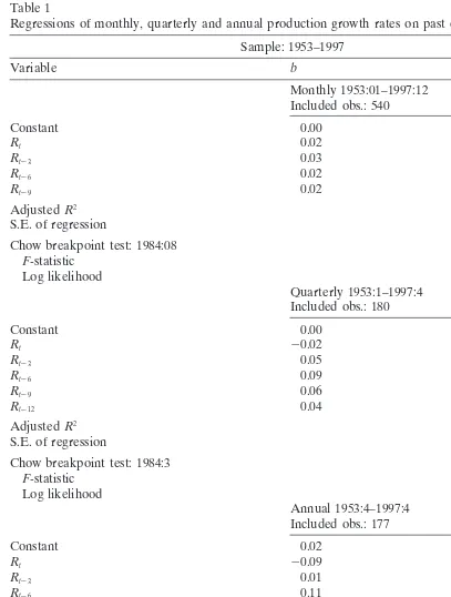
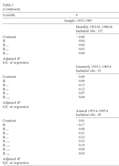
The results are displayed in Table 1.

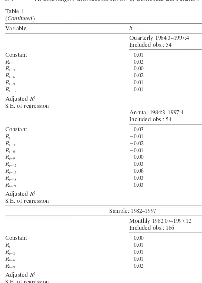
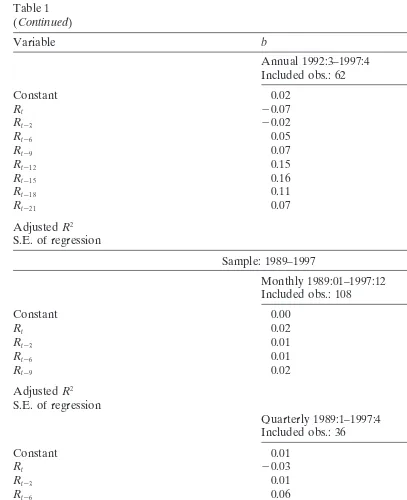
The results for 1953–1997 are close to those for 1953–1987 in Fama (1990, p. 1098, Table II) and the forecasts improve with the time horizon over which production growth is calculated. However, no matter whether we regress monthly, quarterly or annual production growth rates on past returns, they do not possess explanatory power over the subsample from 1984 to 1997. The adjustedR2_{in all regressions are around}

zero and the estimated coefficients are not significant according tot-statistics. Further-more, Chow breakpoint tests indicate a significant subsample instability in 1984 for all regressions. Regressions over the subsample from 1953 to 1965, on the other hand, lead to quite similar results as regressions over the whole sample from 1953 to 1997. Therefore, the two stock market growth periods appear to be fundamentally different because the first stock market growth period seems to have been driven by expectations on real activity, while this cannot be confirmed for the second growth period that started in the early 1980s.

Moreover, the outcome of the regressions using the 1982–1997 sample in Table 1 illustrates the strong influence of the observations in 1983 on the regression parameters. The strong correlation between stock returns and subsequent changes in production growth rates during the early 1980s leads to results that are similar to the results of the regressions using the 1953–1997 sample. From using a sample that includes the observations of 1983 one is not able to detect the change in the relation between stock returns and real activity that seems to have occurred in 1984.

The results of regressions using the 1989–1997 subsample, however, confirm the results of the 1984–1997 sample except for the regression using monthly production growth rates.4_{The values of the adjusted}_R2_{in the regressions of production growth}

rates on past stock returns are small (0.05) for quarterly growth rates and negative (2_{0.18) in the regressions using annual growth rates. Similar to the 1984–1997 period,}

(6)

Table 1

Regressions of monthly, quarterly and annual production growth rates on past quarterly stock returns Sample: 1953–1997

Variable b t(b)

Monthly 1953:01–1997:12 Included obs.: 540

Constant 0.00 1.62

Rt 0.02 2.46

Rt23 0.03 3.34

Rt26 0.02 3.39

Rt29 0.02 3.43

AdjustedR2 _0.12

S.E. of regression 0.01

Chow breakpoint test: 1984:08

F-statistic (0.01)

Log likelihood (0.01)

Quarterly 1953:1–1997:4 Included obs.: 180

Constant 0.00 2.26

Rt 20.02 21.04

Rt23 0.05 3.41

Rt26 0.09 4.55

Rt29 0.06 4.36

Rt212 0.04 3.34

AdjustedR2 _0.27

F-statistic (0.05)

Annual 1953:4–1997:4 Included obs.: 177

Constant 0.02 2.86

Rt 20.09 22.76

Rt23 0.01 0.24

Rt26 0.11 2.79

Rt29 0.19 5.43

Rt212 0.24 6.37

Rt215 0.22 6.67

Rt218 0.12 3.93

Rt221 0.05 1.66

AdjustedR2 _0.39

F-statistic (0.01)

(7)

Table 1 (Continued)

Variable b t(b)

Sample: 1953–1965

Constant 2_0.00 2_0.03

Rt 0.04 2.61

Rt23 0.04 1.54

Rt26 0.03 2.17

Rt29 0.00 0.20

AdjustedR2 _0.11

Constant 0.00 0.11

Rt 0.00 0.09

Rt23 0.13 2.01

Rt26 0.12 1.93

Rt29 0.07 1.96

Rt212 0.00 0.08

AdjustedR2 _0.20

Constant 0.01 0.39

Rt 20.17 21.71

Rt23 0.08 0.71

Rt26 0.21 1.48

Rt29 0.33 2.28

Rt212 0.32 2.27

Rt215 0.19 2.45

Rt218 0.09 0.87

Rt221 0.02 0.17

AdjustedR2 _0.33

Sample: 1984–1997

Constant 0.00 1.72

Rt 0.01 1.29

Rt23 0.00 0.21

Rt26 0.01 1.05

Rt29 0.01 0.70

AdjustedR2 _0.01

(8)

(9)

Variable b t(b)

Constant 0.02 1.35

Rt 20.07 21.39

Rt23 20.02 20.56

Rt26 0.05 0.82

Rt29 0.07 1.16

Rt212 0.15 2.44

Rt215 0.16 2.68

Rt218 0.11 2.56

Rt221 0.07 2.11

AdjustedR2 _0.30

Sample: 1989–1997

Constant 0.00 0.54

Rt 0.02 2.28

Rt23 0.01 0.68

Rt26 0.01 0.53

Rt29 0.02 1.90

AdjustedR2 _0.10

Constant 0.01 1.09

Rt 20.03 21.19

Rt23 0.01 0.33

Rt26 0.06 1.58

Rt29 0.02 0.46

Rt212 0.01 0.41

AdjustedR2 _0.05

Constant 0.02 0.95

Rt 0.06 0.95

Rt23 0.03 0.26

Rt26 0.06 0.54

(10)

Variable b t(b)

Rt29 0.02 0.14

Rt212 0.11 0.97

Rt215 0.06 0.87

Rt218 0.04 0.89

Rt221 0.02 0.75

AdjustedR2 ₂_0.18

The production growth rate is from periodt2_T_to_t_{, and therefore, depending on}_T_{, denotes the} monthy (T5_{1), quarterly (}_T5_{3) or annual (}_T5_{12) production growth rate.}_R

t23k13is the continuously compounded value weighted real return for the quarter fromt2₃_k_to_t2₃_k1_{3. The}_t_{s for the slopes} in all regressions use standard errors that are adjusted for heteroscedasticity and residual autocorrelation by using the method of Newey and West (1987). The Chow breakpoint test gives the significance level of theF-test and the log likelihood test at which the null hypothesis of no subsample instability can be rejected.

Obs.5_{observations; S.E.}5_{standard error.}

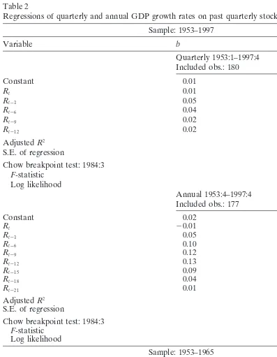
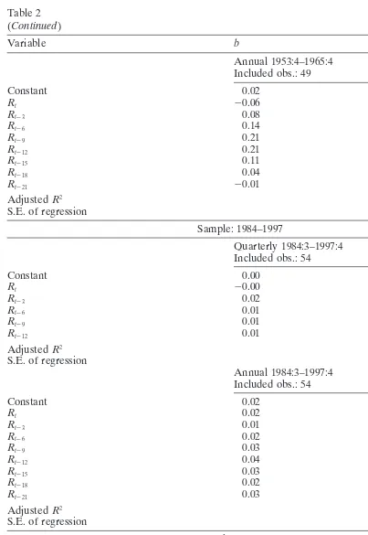
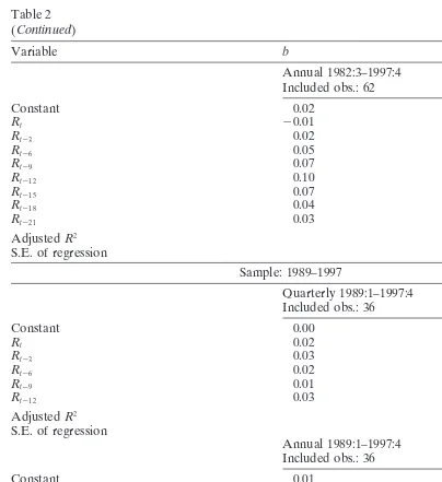
Analogous to Eq. (2), we also run regressions of quarterly and annual real GDP growth rates on past quarterly returns (Table 2).

The results are very close to the regressions of production growth rates on past returns. There is absolutely no relation between past returns and real GDP growth rates (adjustedR2_{zero or below zero) over the 1984–1997 subsample, while the relation}

is especially strong over the subsample from 1953 to 1965. And Chow breakpoint tests indicate a structural break in 1984.

The results of the regressions using the 1989–1997 sample in Table 2 further confirm findings of the regressions using production growth rates over the same period (Table 3) if one looks at the results of the regressions using annual GDP growth rates. A significant correlation between GDP growth rates and subsequent stock returns cannot be detected neither in the 1984–1997 sample nor in the 1989–1997 sample. However, the evidence from the regressions using quarterly GDP growth rates is less clear, because the forecasting power of stock returns increases again when the starting date of the current stock market boom is changed from 1984 to 1989.

(11)

Table 2

Regressions of quarterly and annual GDP growth rates on past quarterly stock returns Sample: 1953–1997

Variable b t(b)

Constant 0.01 4.43

Rt 0.01 1.46

Rt23 0.05 3.91

Rt26 0.04 4.32

Rt29 0.02 1.79

Rt212 0.02 3.06

AdjustedR2 _0.23

F-statistic (0.04)

Constant 0.02 5.03

Rt 20.01 20.45

Rt23 0.05 2.79

Rt26 0.10 4.53

Rt29 0.12 5.69

Rt212 0.13 6.59

Rt215 0.09 5.57

Rt218 0.04 2.01

Rt221 0.01 0.55

AdjustedR2 _0.32

F-statistic (0.01)

Sample: 1953–1965

Constant 0.00 1.40

Rt 0.01 0.30

Rt23 0.10 2.57

Rt26 0.05 2.27

Rt29 0.04 2.39

Rt212 0.01 0.89

AdjustedR2 _0.35

(12)

(13)

Table 2

The GDP growth rate is from periodt2_T_to_t_{, and, therefore, depending on}_T_{, denotes the quarterly} (T5_{3) or annual (}_T5_{12) GDP growth rate.}_R

t23k13is the continuously compounded value weighted real return for the quarter fromt2₃_k_to_t2₃_k1_{3. The}_t_{s for the slopes in all regressions use standard} errors that are adjusted for heteroscedasticity and residual autocorrelation by using the method of Newey and West (1987). The Chow breakpoint test gives the significance level of theF-test and the log likelihood test at which the null hypothesis of no subsample instability can be rejected.

(14)

3. Expected returns and real activity

As indicated in the introductory section, there are two channels through which real activity is supposed to be connected to stock returns. The first channel is the positive effect of expected growth rates of real activity on future cash flows which, in turn, increases stock prices (and stock returns) according to standard valuation models. This channel, however, seems to be insignificant since 1984 according to our tests in the previous section. The second channel, which we will investigate in this section, is the forecastable variation of future returns by variables that correlate with current business conditions and, therefore, current real activity. The most popular of these variables are the dividend yield and differences between various interest rates such as the default spread or the term spread, which several studies found to be able to forecast returns (e.g., Chen, 1991; Fama, 1990; Fama & French, 1989; Patelis, 1997; Schwert, 1990). The commonly held view among these authors is that the variations in expected returns are rational variations in response to business conditions.

The influence of real activity through the dividend yield or interest spreads involves some theoretical considerations from intertemporal market equilibrium models as developed by Cox, Ingersoll, and Ross (1985) and others. These models imply that stock returns are negatively related to recent growth of GDP as has been especially outlined by Chen (1991). Stock prices and, therefore, expected returns are interpreted as functions of current business conditions as indicated by recent GDP growth rates. If the economy is in a depressed state because income growth has been poor (and also wealth is low), investors will save less and move consumption from the future to the present (consumption smoothing). This behavior can be explained by consumption functions where risk aversion increases with decreasing levels of income.5

Conse-quently, they will demand a higher risk premium if income decreases, as the risk pre-mium of the market is a positive function of the aggregate risk aversion. Based on these considerations, Chen (1991) draws the conclusion that, if we take the recent growth rate of the economy as a proxy for the current health of the economy, risk premiums and, therefore, expected market returns should show negative correlations with the recent growth rate.6

(15)

To investigate whether stock returns and real activity are still connected through the effect on expected returns during the current stock growth period, we have to examine for two different things: whether the variables proxying for expected stock returns are indeed able to forecast stock returns and, if this is the case, if the fore-castability is due to their correlation with current business conditions. Therefore, we first run regressions of stock returns on the forecasting variables including regressions that also involve future production growth rates. Then, we will examine the relation between the forecasting variables and business conditions by running regressions of production and real GDP growth rates on the forecasting variables.

The variables used to forecast stock returns are calculated as follows:

1. The dividend yield (DYt) is constructed from the CRSP stock return series, with and without dividends, as in Hodrick (1992). Normalized nominal stock prices are obtained by setting the stock price (Pt) equal to one in the first month of the sample period, and recursively setting Pt 5 (1 1 RXt)Pt2₁, where RXt is equal to value-weighted returns without dividends. Then the dividend yield (DYt) for each month is calculated by summing monthly dividends for the year preceding taccording to Eq. (3):

DYt5

o

11

i50

(RDt2i2RXt2i)Pt2i

Pt

, (3)

whereRDtstands for value weighted returns with dividends.

2. TERMtis the term spread between ten-year treasury bonds and the federal funds rate (data from Federal Reserve Board) which differs from Fama (1990), who uses the difference between the annual yield on Aaa corporate bonds and the one-month treasury bill yield. However, the results are only slightly different from the results obtained in Fama (1990) if one tests for a sample from 1954–1987. 3. FFRt is the federal funds rate. As according to unit roots tests the unit root hypothesis can not be rejected for this variable, the first difference of the federal funds rate (DFFRt) is used in the following tests.

Fama and French (1989) find that the dividend yield and the default spread capture similar variation in expected return. Therefore, it does not make sense to include both variables in the same regressions. Fama (1990) runs all regressions twice, once with the dividend yield and once with the default spread which basically leads to the same results. As the dividend yield generally seems to be a more powerful and more robust predictor of expected return variation, as shown in a recent article by Patelis (1997), we will concentrate on the dividend yield and on the term spread as our forecasting variables. Additionally, we also include the federal funds rate as an indica-tor of monetary policy in our tests.7_{Fama and French (1989) argue that the behavior}

(16)

related to monetary policy and may correlate with stock returns because they proxy for the stance of monetary policy as well as for current business conditions.

As the term spread and federal funds rate series used here start in August of 1954, we run the following regressions for the sample from 1954 to 1997 and the 1984–1997 subsample [Eq. (4)].

Rt1T 5a 1b1DYt1b2SPREADt1 b3DFFRt1 et (4)

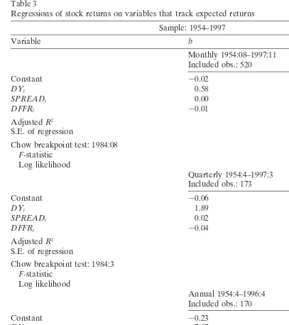
whereTstands for a period of one, three or twelve months. Again, following Fama (1990) we first run regressions of stock returns on the variables proxying for expected stock returns of the following form (Table 3).8

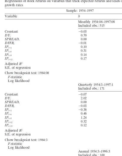
As in Fama (1990, p. 1100, Table IV) the dividend yield and the term spread forecast stock returns over the full sample from 1954 to 1997 and also changes in the federal funds rate seem to be somewhat significant according to t-statistics for regressions using monthly and quarterly returns. The forecasting ability increases with the time horizon over which returns are measured as before in the regressions of stock returns on production growth rates.

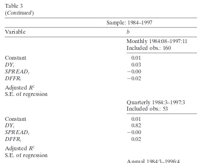
If we run the same regressions for the 1984–1997 subsample, the forecasting ability is much weaker. The adjustedR2_{are even negative for quarterly and annual returns}

and none of the estimated coefficients for the dividend yield, the term spread and the first difference of the federal funds rate is significant according to t-statistics. Moreover, Chow breakpoint tests suggest a significant breakpoint in 1984 in the re-gressions using monthly and annual returns. Running the same rere-gressions for the 1989–1997 subsample (results not reported here) leads to very similar results as the regressions over the 1984–1997 sample. The values of the adjustedR2_{are around zero}

and none of the estimated coefficients is significant.

Next, we also add production growth rates to the regressions in order to test whether the forecasting variables proxying for expected return variation and future production growth rates proxying for forecasts of real activity possess independent explanatory power. Table 4 contains estimates of the regression [Eq. (5)]:

Rt1T 5a 1b1DYt1b2SPREADt1 b3DFFRt1

o

8

k51

bk13IPt13k 1 et (5)

where, again,Tstands for a period of one, three or twelve months.

For the whole sample (1954–1997), the results are close to Fama (1990, pp. 1102– 1103, Table V). Future production growth rates forecast stock returns over several quarters as is most evident from the regression using annual returns. The dividend yield shows considerable forecasting power in all regressions that also include future production growth rates, while the term spread is only significant in the regression using annual returns and changes in the federal funds rate are insignificant. This confirms previous findings that the dividend yield is able to track variations in future stock returns which are, at least to some degree, independent of variations explained by future production growth rates and vice versa.9 _{The decline in the explanatory}

(17)

Table 3

Regressions of stock returns on variables that track expected returns Sample: 1954–1997

Variable b t(b)

Constant 2_0.02 2_1.95

DYt 0.58 2.37

SPREADt 0.00 3.79

DFFRt 20.01 21.83

AdjustedR2 _0.04

F-statistic (0.02)

Constant 2_0.06 2_1.57

DYt 1.89 2.01

SPREADt 0.02 2.67

DFFRt 20.04 22.16

AdjustedR2 _0.10

F-statistic (0.15)

Constant 2_0.23 2_1.78

DYt 7.67 2.36

SPREADt 0.04 2.57

DFFRt 20.05 21.88

AdjustedR2 _0.20

F-statistic (0.00)

(continued)

also include future production growth rates suggests correlation with future production growth rates, which is confirmed by the results displayed in Table 6.

(18)

Sample: 1984–1997

Variable b t(b)

Constant 0.01 2_0.69

DYt 0.03 0.06

SPREADt 20.00 20.76

DFFRt 20.02 21.81

AdjustedR2 _0.01

Constant 0.01 0.21

DYt 0.82 0.56

SPREADt 20.00 20.37

DFFRt 0.02 0.43

AdjustedR2 2_0.05

Constant 0.02 0.13

DYt 2.11 0.41

SPREADt 0.02 0.75

DFFRt 20.02 20.22

AdjustedR2 2_0.03

DYtstands for the dividend yield,TERMtis the term spread between 10-year treasury bonds and the federal funds rate, andDFFRtis the first difference of the federal funds rate. Thets for the slopes in all regressions use standard errors that are adjusted for heteroscedasticity and residual autocorrelation by using the method of Newey and West (1987). The Chow breakpoint test gives the significance level of theF-test and the log likelihood test at which the null hypothesis of no subsample instability can be rejected.

Obs.5_{observations; S.E.}5_{standard error.}

the 1984–1997 subsample (Table 4). Over the 1953–1965 subsample the combined forecasting power of the dividend yield and future production growth rates is similar to the forecasting power over the 1954–1997 sample and it is especially strong for the regressions using annual returns where the adjustedR2_{is 0.68. The regressions over}

the 1984–1997 subsample, on the other hand, lead to considerably lower adjustedR2

(19)

Table 4

(20)

Variable b t(b)

AdjustedR2 _0.45

F-statistic (0.00)

Sample: 1953–1965

Constant 2_0.04 2_2.50

DYt 1.03 2.88

IPt13 0.27 2.89

IPt16 0.19 2.03

IPt19 0.17 1.81

IPt112 0.02 0.24

AdjustedR2 _0.10

Constant 2_0.11 2_2.43

DYt 3.27 2.81

IPt13 0.14 0.36

IPt16 0.83 2.12

IPt19 0.65 1.59

IPt112 0.29 0.72

IPt115 0.03 0.06

AdjustedR2 _0.25

Constant 2_0.45 2_4.93

DYt 12.70 6.24

IPt13 20.03 20.07

IPt16 0.95 2.32

IPt19 1.50 3.74

IPt112 1.53 3.48

IPt115 1.55 3.55

IPt118 0.90 2.79

IPt121 0.94 1.89

(21)

Table 4

DYtstands for the dividend yield,TERMtis the term spread between 10-year treasury bonds and the federal funds rate, andDFFRtis the first difference of the federal funds rate.IPt13kis the production growth rate from periodttot1₃_k_{. The}_t_{s for the slopes in all regressions use standard errors that are} adjusted for heteroscedasticity and residual autocorrelation by using the method of Newey and West (1987). The Chow breakpoint test gives the significance level of theF-test and the log likelihood test at which the null hypothesis of no subsample instability can be rejected.

(22)

Table 5

(23)

Lead 1953:1–1997:4 1953:1–1965:4 1984:3–1997:4

(2) 2_0.55 2_0.93 2_0.47

(2_3.10) ₍2_1.72) ₍2_3.05)

0.05 0.05 0.14

(0.17)

(3) 2_0.28 2_0.51 2_0.52

(2_1.51) ₍2_0.77) ₍2_3.20)

0.01 0.00 0.15

(0.55)

The slope coefficient (b) and the t-ratios (in parentheses) are adjusted for heteroscedasticity and residual autocorrelation by using the method of Newey and West (1987), with the adjustedR2_{for the} corresponding regression. The last number (in parentheses) of the tests for the full sample (1953–1997) presents the probability of the Chow breakpoint test (F-statistic) at which the null hypothesis of no subsample instability can be rejected for the third quarter of 1984.

We now turn to the question whether variables proxying for expected stock returns in fact show a statistically significant correlation with real activity. Therefore, in a fashion similar to Chen (1991)10_{we relate the dividend yield and the term spread to}

past, current, and future quarterly growth rates of real activity as represented by GDP and production growth rates and run the univariate regressions [Eqs. (6) and (7)]

GDPt1lead5 a1bXt1 et (6)

IPt1lead5 a1bXt1 et (7)

whereXtstands forDYt(Table 5) andSPREADt(Table 6).

The regressions over the full sample (1953–1997 forDYt) in Table 5, lead to results that are very similar to the ones reported in Chen (1991, pp. 538–539, Table IV), who runs the same regressions for the period from 1954 to 1985. The dividend yield shows significant negative correlation with GDP growth rates over the quarters fromt2₂

tot11 and with production growth rates over the quarters from_t21 to_t12. The

(24)

Table 6

(25)

Lead 1954:3–1997:4 1984:3–1997:4

(3) 0.005 0.002

(5.40) (1.95)

0.14 0.05

(0.00)

(4) 0.004 0.002

(4.15) (1.98)

0.09 0.05

(0.08)

(5) 0.003 0.002

(3.31) (2.41)

0.06 0.09

(0.28)

The slope coefficient (b) and the t-ratios (in parentheses) are adjusted for heteroscedasticity and residual autocorrelation by using the method of Newey and West (1987), with the adjustedR2_{for the} corresponding regression. The last number (in parentheses) of the tests for the full sample (1954–1997) presents the probability of the Chow breakpoint test (F-statistic) at which the null hypothesis of no subsample instability can be rejected for the second quarter of 1984.

The results suggest that, in spite of the absence of significant correlations between GDP growth rates and the dividend yield in the 1984–1997 subsample, the dividend yield continued to be an indicator of business conditions also after 1984. However, the correlations seem to be somewhat different after 1984. While the correlations with past GDP growth rates and past production growth rates seem to have disappeared, the dividend yield now significantly correlates with future growth rates of production and GDP. This change is also reflected in the results of Chow breakpoint tests that confirm a significant breakpoint in the third quarter of 1984 in most of the univariate regressions (Table 5). Since the early 1980s, the dividend yield seems to have turned from a backward-looking indicator into a significant predictor of future real economic activity over several quarters.

If we look at the relation between the term spread and real activity (Table 6) the results for the full sample (1954–1997) are also close to Chen’s (1991) results. Contrary to the dividend yield, the time spread is not supposed to correlate with past and current GDP or production growth rates, but with future growth rates. We find that a higher term spread forecasts higher GDP and production growth rates for the next five quarters, which supports the findings in Chen (1991). This result is not fundamentally changed in the 1984–1997 sample. The term spread remains a significant predictor of future real activity, no matter whether GDP or production is used as a measure of real activity. However, the forecasting pattern in the 1984–1997 subsample is slightly different as also indicated by the results of the Chow breakpoint tests, which suggest a significant breakpoint (at the 1% level) in the third quarter of 1984 in most of the univariate regressions.

(26)

through which real activity is supposed to be connected to stock returns, became doubtful in the 1984–1997 subsample. The dividend yield as well as the term spread continue to show significant correlations with business conditions in the 1984–1997 subsample. Therefore, variations in expected returns in response to the dividend yield and the term spread would still have been rational in this period. But as the regressions in this section showed (Tables 3 and 4), such variations cannot be detected. Conse-quently, the lack of forecasting power of these indicators in the 1984–1997 sample adds further evidence to the previous finding that stock returns do not reflect real activity in the current stock market boom.

4. Conclusions

Regressions of stock returns on measures of real activity in the United States over the period from 1953 to 1997 seem to confirm previous findings of Fama (1990) and others: a large fraction of stock return variations can be explained by future values of measures of real activity. However, things look quite different if the regressions are run over a subsample covering the recent boom on the stock market since the early 1980s. This article presents evidence that there is a breakdown in the relation between stock returns and future real activity in the U.S. economy since the early 1980s. This result holds up no matter whether one uses monthly, quarterly or annual real stock returns, whether real activity is represented by production growth rates or real GDP growth rates or whether the 1987 episode is included or excluded from the regressions. Current stock returns do not seem to contain significant information about future real activity as before. However, because the 1984–1997 period as well as the 1989–1998 period—which we found to be characterized by the absence of a relation between stock returns and future real activity—are rather short we cannot be sure yet whether the result should be interpreted as a temporary aberration or whether it is of a permanent nature. But, the difference to the results of regressions over the 1953–1965 subsample that represents the first high growth period is obvious. Then, correlations between stock returns and subsequent real activity were significant, while the present high growth period is characterized by an absence of these correla-tions that according to Schwert (1990) used to hold for the whole century.11

Further evidence for deviations from the fundamental value comes from regressions of stock returns on the dividend yield and the term spread. Both of these variables are supposed to track expected returns due to their correlation with past and present (dividend yield) or future (term spread) growth rates of real activities. According to our regressions, these variables still correlate with business conditions after 1984, although the dividend yield seems to correlate more with future real activity and less with past real activity since 1984. Consequently, because the relation between stock returns and future real activity broke down, the dividend yield and the term spread cannot track stock returns in the 1984–1997 subsample any longer. Forecastable varia-tion in future returns on the stock market in response to changing business condivaria-tions also seem to be absent in the current stock market boom.

(27)

early 1980s, is fundamentally different from the first high stock growth period from the late 1940s to the mid 1960s, although measures of stock market valuations such as the ratio of market value of shares to GDP or the price dividend ratio show a similar pattern over the two high growth episodes. But, during the first high growth period correlations between stock returns and subsequent growth rates of real activity were significant, while this correlation cannot be detected in the data covering the second high growth period. Possible sources of explanation of this finding are discussed in Binswanger (1999), where the emergence of persistent speculative bubbles since the early 1980s is highlighted as a plausible cause. However, further research is needed in order to uncover the exact nature of the recent stock market boom. Using stock returns and industrial production data cut by industry may also provide additional insights.

Acknowledgments

The author would like to thank Marcel Savioz, as well as two anonymous referees for helpful suggestions and comments.

Notes

1. Of course, as outlined in Barro (1990) and Fama (1990), stock returns and production growth rates may also be both affected by other variables such as interest rates and not all changes in stock returns are caused by information on future cash flows in production. A fall in the interest rate (and therefore the rate that is used to discount future cash flows) can cause an increase in stock prices as well as an increase in future production. And, raising stock prices increase wealth which may stimulate future demand for consumption and investment goods. These non-mutually exclusive hypotheses also suggest a correlation between future production growth rates and current stock returns. But, they further support the argument that stock prices should lead real activity. 2. These tests are included in the extended working paper version of this article,

which is available from the author upon request.

3. The first test in Fama (1990, p. 1096) is a regression of monthly production growth rates on lagged monthly stock returns. However, production growth rates are not well predicted by monthly returns as the period of one month appears to be too short (see Note 4). Therefore, results are nor reported here. 4. As explained in Fama (1990, p. 1097), lagged returns are noisy forecasts of monthly production growth rates because information about the production of a given month is spread over many past periods. Therefore, we will mainly base our interpretations on the regressions using quarterly and annual growth rates where the forecasting power is much higher.

(28)

6. A fact, many times ignored by theoretical models, is that much of the investing in the stock market is done by institutional investors and that a large fraction of the stocks directly held by households are actually held by a small, wealthy segment of the population (Shiller, 1995). Therefore, consumption decisions of the largest part of the population leaves stock returns virtually unaffected and one has to study how the consumption of the wealthy segment directly owning stock correlates with stock returns as it is, for example, done in Mankiw and Zeldes (1991).

7. According to Bernanke and Blinder (1992) the federal funds rate is a good indicator of monetary policy actions because it is sensitive to shocks to the supply of bank reserves. At least this seems to be true for the time period before 1979 and also after the mid-1980s (Bernanke & Mihov, 1995).

8. Fama (1990) additionally also includes variables that proxy for shocks to the default spread and the term spread. However, only shocks to the default spread appear to be somewhat significant.

9. As shown in Fama (1990), the same is also true for the default spread, whose forecasting power is not examined here.

10. Chen (1991) uses gross national product (GNP) instead of GDP growth rates and does not test whether the forecasting variables correlate with production growth rates. He interprets the production growth rate itself as a state variable that varies with business conditions (as indicated by GNP growth) and finds that production growth rates are leading GNP growth rates.

11. These results, however, are only valid for a forecasting horizon of up to two years and do not say anything about longer term forecastability over moving averages of several years or decades as, for example, studied in Barsky and De Long (1993) or Campbell and Shiller (1998).

References

Barro, R. (1990). The stock market and investment.Review of Financial Studies 3, 115–131.

Barsky, R., & De Long, B. (1993). Why does the stock market fluctuate?Quarterly Journal of Economics 108, 293–311.

Bernanke, B., & Blinder, A. (1992). The federal funds rate and the channels of monetary transmission.

American Economic Review 82, 901–921.

Bernanke, B., & Mihov, I. (1995). Measuring monetary policy. NBER Working Paper No. 5145, Cam-bridge, MA.

Binswanger, M. (1999).Stock Markets, Speculative Bubbles and Economic Growth.Cheltenham, UK: Edward Elgar.

Campbell, J., & Shiller, R. (1998). Valuation ratios and the long-run stock market outlook.Journal of

Portfolio Management 24, 11–26.

Chen, N. F. (1991). Financial investment opportunities and the macroeconomy.Journal of Finance 46, 529–554.

Cochrane, J. (1997). Where is the market going? Uncertain facts and novel theories.Economic Perspectives 21, 3–37.

Cox, J., Ingersoll, J., & Ross, S. (1985). An intertemporal general equilibrium model of asset prices.

(29)

Domian, D., & Louton, D. (1997). A threshold autoregresive analysis of stock returns and real economic activity.International Review of Economics and Finance 6, 167–179.

Estrella, A., & Mishkin, F. (1996). Predicting U.S. recessions: financial variables as leading indicators. Federal Reserve Bank of New York research paper no. 9609.

Fama, E. (1981). Stock returns, real activity, inflation, and money.American Economic Review 71, 545–565. Fama, E. (1990). Stock returns, expected returns, and real activity.Journal of Finance 45, 1089–1108. Fama, E., & French, K. (1989). Business conditions and expected returns on stocks and bonds.Journal

of Financial Economics 25, 23–49.

Hodrick, R. (1992). Dividend yields and expected stock returns: alternative procedures for inference and measurement.The Review of Financial Studies 5, 357–386.

Ibbotson, R. (1994).Yearbook.Chicago: Ibbotson Associates.

Lee, B. S. (1992). Causal relations among stock returns, interest rates, real activity, and inflation.Journal of Finance 47, 1591–1603.

Mankiw, G., & Zeldes, S. (1991). The consumption of stockholders and non-stockholders.Journal of

Financial Economics 29, 97–112.

Morck, R., Shleifer, A., & Vishny, R. (1990). The stock market and investment: is the market a sideshow?

Brookings Papers on Economic Activity 1, 157–202.

Newey, W., & West, K. (1987). A simple, positive semi-definite, heteroscedasticity and autocorrelation consistent covariance matrix.Econometrica 55, 703–708.

Patelis, A. (1997). Stock return predictability: the role of monetary policy.Journal of Finance 52, 1951–1972. Peiro, A. (1996). Stock prices, production and interest rates: comparison of three European countries

with the USA.Empirical Economics 2, 221–234.

Schwert, W. (1990). Stock returns and real activity: a century of evidence.Journal of Finance 45, 1237–1257. Shapiro, M. (1988). The stabilization of the U.S. economy: evidence from the stock market.American

Economic Review 78, 1067–1079.