q
The"rst two authors are with the Research Department of the International Monetary Fund. The third author is at the Stockholm School of Economics. We are grateful for comments received from Lars Svensson, from participants at the Computational Economics Symposium at Cambridge University (June 29}July 1, 1998) and the Reserve Bank of New Zealand Conference on Monetary Policy Under Uncertainty (June 29}July 3, 1998), and from an anonymous referee. The views expressed in this paper are those of the authors and do not necessarily re#ect those of the International Monetary Fund.
*Corresponding author. Tel.: (202)623-6640; fax: (202)623-6334. E-mail address:[email protected] (P. Isard).
25 (2001) 115}148
In#ation targeting with NAIRU uncertainty
and endogenous policy credibility
qPeter Isard
*
, Douglas Laxton, Ann-Charlotte Eliasson
Research Department, International Monetary Fund, Washington, DC 20431, USA
Accepted 9 November 1999
Abstract
Stochastic simulations are employed to compare performances of monetary policy rules in linear and nonlinear variants of a small macro model with NAIRU uncertainty under di!erent assumptions about the way in#ation expectations are formed. Cases in which policy credibility is ignored or treated as exogenous are distinguished from cases in which credibility and in#ation expectations respond endogenously to the monetary authorities'track record in delivering low in#ation. It is shown that endogenous policy credibility strengthens the case for forward-looking in#ation forecast based rules relative to backward-looking Taylor rules. ( 2001 Elsevier Science B.V. All rights reserved.
JEL classixcation: C51; E31; E52
Keywords: In#ation targeting; Monetary policy rules; Credibility; NAIRU uncertainty
1Finland and Spain also operated with quantitative in#ation targets for several years prior to relinquishing monetary policymaking to the European Central Bank.
2See, for example, Fischer (1996), Freedman (1996), Svensson (1997), Bernanke and Mishkin (1997) and Debelle (1997).
3A number of recent examples of such papers were included in the programs of the NBER Conference on Monetary Policy Rules (January 15}17, 1998), the Federal Reserve Bank of San Francisco Conference on Central Bank In#ation Targeting (March 6}7, 1998), the Bank of Sweden Conference on Monetary Policy Rules (June 12}13, 1998), the 1998 Symposium on Computational Economics at Cambridge University (June 29}July 1, 1998), and the Reserve Bank of New Zealand Conference on Monetary Policy Under Uncertainty (June 29}July 3, 1998). Earlier contributions to the in#ation targeting literature include the conference volumes Leiderman and Svensson (1995), Haldane (1995), Federal Reserve Bank of Kansas City (1996), and Lowe (1997).
4Rudebush and Svensson (1999) and Svensson (1999) distinguish between reaction functions that are essentially derived as"rst-order conditions for minimizing policy loss functions and reaction functions that are simply postulated, suggest that the term&targeting rule'should only be applied to the former class of reaction functions.
5See, for example, Levin et al. (1999) and Taylor (1999). 1. Introduction
In#ation targeting has become a popular monetary policy strategy for indus-trial countries. Quantitative targets or target ranges for in#ation have been announced by New Zealand (in 1990), Canada (1991), Israel (1991), the United Kingdom (1992), Australia (1993), and Sweden (1993),1while a number of other countries have implemented strategies that emphasize informal objectives for in#ation. In describing the attractiveness of such strategies, proponents have emphasized that an in#ation targeting framework can make the objectives of monetary policy more transparent and, over time, may result in an increase in policy credibility that in turn has desirable implications for macroeconomic performance.2
6For example, Batini and Haldane (1999), Amano et al. (1999), and Rudebusch and Svensson (1999).
7Taylor (1993, p. 213).
8Related to this point, the issue of rules versus discretion for monetary policy has become less actively debated during the 1990s. This may re#ect,"rst, a general acceptance of the premise that a fully-state-contingent rule for monetary policy is not a relevant possibility in a world in which knowledge about the macroeconomic structure and the nature of disturbances is incomplete, and second, a general awareness of the fact that simple (or partially-state-contingent) rules and discretion cannot be unambiguously ranked. In this context, Flood and Isard (1989,1990) suggested that
rules can be outperformed by rules in which interest rates are adjusted in response to both the output gap and the deviation from target of an in#ation
forecast(rather than the deviation from target of the current in#ation rate).6We follow the terminology of Batini and Haldane (1999) and Amano et al. (1999) in referring to the latter type of reaction functions as in#ation forecast based (IFB) rules. Such rules have the feature of inducing the authorities to base their interest rate settings on the determinants of (future) in#ation, given their informa-tion/assumptions about the macroeconomic model.
Economists confront a fundamental di$culty when attempting to analyze how monetary policy strategies should be formulated. On the one hand, the challenge of addressing the relevant issues with coherence and depth requires a formal model that speci"es the relationships between the instrument variables that the monetary authorities control and the target variables that are used to evaluate macroeconomic performance. Analysis of the hypothetical perfor-mances of mechanical rules within simple but fairly realistic macroeconomic models can provide valuable guidance about the types of policy reactions that are likely to be relatively e!ective for achieving and maintaining macroeco-nomic stability in the real world. On the other hand, the &true model' of the relationships between policy instruments and targets is much more complex than economists can hope to formalize, not only because it is di$cult to model the aggregate behavior of large numbers of heterogeneous economic agents, but also because the behavior of individual agents evolves over time with innova-tions in information technologies, the introduction of new markets and prod-ucts, changes in"scal and structural policies, and so forth.
footnote 8 continued
monetary authorities should be given incentives to follow simple rules with&escape clauses', in recognition of the tradeo!between the various bene"ts of rules and the social costs of failing to modify reaction functions in certain unforeseeable circumstances. Amano et al. (1999), among others, emphasize that credibility is a two-edged sword, and that the credibility bene"ts of monetary policy rules cannot be e!ectively reaped unless the monetary authorities are prepared to change their reaction function over time in response to new information about macroeconomic structure.
9McCallum (1988).
10In#ation expectations are often modeled as a weighted sum of backward- and forward-looking components, and in this context a number of studies have followed Freedman (1996) in de"ning the forward-looking component as the announced in#ation target and in interpreting the weight on this component as a measure of policy credibility. Within this framework, Amano et al. (1999) have analyzed the implications for monetary policy of&exogenous'changes in credibility. In addition, Tetlow et al. (1999) have analyzed the optimal form of simple rules when private agents have to learn about the rule. To our knowledge, however, few if any evaluations of policy reaction functions have modeled credibility as a variable that responds endogenously to the monetary authority's perfor-mance in delivering macroeconomic stability.
11See, for example, Isard and Laxton (1996), Clark and Laxton (1997), and Laxton et al. (1999). See also Summers (1988), who questioned the value of basing policy analysis on models in which monetary policy is incapable of in#uencing the average rates of in#ation and unemployment.
12We report simulations for two calibrations of each class of rules. The"rst corresponds to the calibration suggested in Taylor (1993); the second is based on a calibration suggested by our analysis in Isard and Laxton (1999).
13For most of the equations the sample period runs from the early 1980s through the mid-1990s.
The unknowability of the true macroeconomic model has also led to the view that the evaluation of policy rules should focus on the robustness of their performances across di!erent classes of plausible models.9Our point of depar-ture for this paper is the observation that progress in the search for robustness has been de"cient in several dimensions. In particular, most tests of monetary policy rules have been performed using models that abstract from endogenous policy credibility,10 that make unrealistically strong assumptions about the monetary authority's knowledge of the NAIRU, and that ignore possible con-vexity of the short-run Phillips curve. These de"ciencies require attention. Most central bankers regard endogenous policy credibility and NAIRU uncertainty as fundamental characteristics of the worlds in which monetary policy must be conducted, and we regard convex short-run Phillips curves as considerably more plausible than linear Phillips curves and as a strategically more appropri-ate assumption for policy analysis.11
14Orphanides (1999) constructs a database of the information available to U.S. policymakers in real time from 1965 to 1993 and suggests that misperception of the economy's productive capacity was the primary underlying cause of the in#ation of the 1970s.
15See Smets (1999) and Drew et al. (1999) for other analyses of the implications of uncertainty about the NAIRU (or the output gap).
16In the linear variants of our model, the degree to which IFB rules outperform Taylor rules appears to be slightly greater under forward-looking expectations than under backward-looking expectations. This contrasts with results from other models, in which the optimal degree of forward-lookingness in the policy rule has been shown to depend on the degree of backward-lookingness in expectations, which is often associated with the length of contract lags in wage and price setting; see, for example, Batini and Haldane (1999).
combinations of linear and nonlinear short-run Phillips curves with di!erent assumptions about the way the public forms its in#ation expectations. We distinguish three cases of in#ation expectations: backward-looking expectations under which credibility is ignored; forward-looking expectations that treat credibility as exogenous; and a forward-looking case in which credibility and in#ation expectations respond endogenously to the policy track record in delivering low in#ation.
In practice, monetary policy operates under considerable uncertainty about model parameters, including imprecise estimates of the NAIRU.14 Our com-parisons of monetary policy rules attempt to capture this element of reality by treating the NAIRU as an uncertain and time varying parameter.15 The authorities are assumed to continually update their estimates of the NAIRU based on their continuing observations of unemployment and in#ation and their partial knowledge of the true macroeconomic model. But like all other econom-ists, they inevitably make serially correlated errors in estimating the NAIRU ex ante, so it is important to evaluate monetary policy rules in the realistic context of ongoing policy errors.
17In Isard and Laxton (1999) we focus on a variant of IFB rules in which the authorities react to a weighted average of the deviation from target of their own in#ation forecast and the deviation from target of the public's in#ation forecast (as re#ected in survey measures of in#ation expectations). Monetary rules that give weight to the latter deviation}that is, to the bias in the public's in#ation expectations}would appear to establish a channel for policy to respond directly to changes in credibility.
endogenous policy credibility and/or convex Phillips curves}where monetary policy does have "rst-order welfare e!ects } the forward-looking IFB rules outperform Taylor rules, and the choice among di!erent calibrations of IFB rules or Taylor rules can have substantial implications for the means of unem-ployment and in#ation. One line of intuition is that forward-looking and relatively forceful policy reactions can be particularly important when credibil-ity can be lost much more quickly than it can be regained.17In this connection we show that a popular calibration suggested by Taylor (1993) for the U.S. economy can be improved upon signi"cantly in our model. Additional intuition for the poor performance of Taylor rules relative to IFB rules comes from noting that the performance of a simple linear rule in a nonlinear model can be improved by specifying the rule in terms of a model-consistent forecast that re#ects the nonlinearities in the model.
The paper is organized as follows. Section 2 motivates the treatment of endogenous policy credibility and presents the basic model. Section 3 describes the design of our stochastic simulation experiments and discusses the di!erent policy reaction functions and model variants that we consider. Section 4 assesses the simulation results. Section 5 concludes.
2. A model of the in6ation}unemployment process
2.1. Background
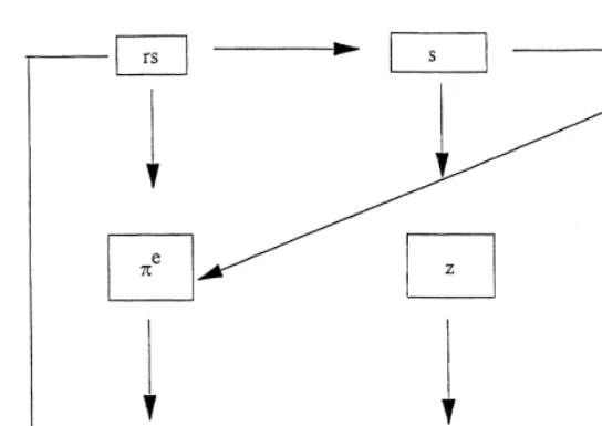
Fig. 1. The monetary policy transmission mechanism.
(n%); changes in the real interest rate in turn in#uence unemployment through their e!ects on aggregate demand and the domestic output gap; and changes in the output gap and unemployment rate in#uence the in#ation rate through channels summarized by the Phillips curve. In addition, an important two-way feedback mechanism is superimposed on the transmission process, with in#ation expectations responding (inter alia) to the history of in#ation, and with in#ation in#uenced in turn by changes in in#ation expectations.
Fig. 1 does not show any feedback from the policy target variables to the policy instrument. The tasks of identifying and implementing a mechanism for reacting to economic developments in a manner that is conducive to macroeco-nomic stability is the responsibility of the monetary authorities. In particular, the role of monetary policy is to adjust the policy instrument variable (in this case the nominal interest rate) in reaction to observed and anticipated changes in unemployment, in#ation, and other macroeconomic variables, taking ac-count of the behavioral relationships among these variables.
the e!ects on macroeconomic variables of various types of economic shocks. In principle, there can be exogenous shocks that directly a!ect the exchange rate, the observed in#ation rate, or the expected in#ation rate; and there can be exogenous shifts in the output gap associated with shocks to either aggregate demand or potential aggregate supply.
The operation of monetary policy is also complicated by the fact that policy credibility is imperfect and can vary with the e!ectiveness of the monetary authorities in achieving desirable outcomes for policy target variables. The endogenous behavior of policy credibility and its role in the monetary policy transmission mechanism has not yet been adequately incorporated into the models that have been used to analyze monetary policy issues.
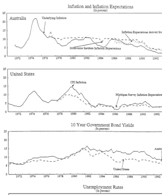
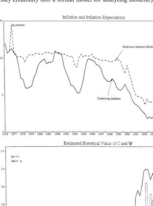
To motivate our interest in exploring the relevance of endogenous policy credibility for the design of monetary policy strategies, Fig. 2 plots quarterly data on selected economic indicators for Australia and the United States. The top two panels show recorded in#ation rates and survey measures of in#ation expectations. In the United States, in#ation has been generally subdued and trendless since the early 1980s, after declining sharply during 1980}1982 in the context of a relatively tight monetary policy. In Australia, in#ation declined more gradually from the levels experienced during the 1970s and has been generally subdued and trendless only since the early 1990s. Survey measures of Australian in#ation expectations have remained persistently above recorded in#ation rates during the past decade, while survey measures of U.S. in#ation expectations have tracked recorded in#ation rates fairly closely. Moreover, with similar recorded in#ation rates in Australia and the United States during the 1990s, long-term Australian government bonds have required an interest pre-mium relative to the yield on U.S. government bonds, as shown in the third panel; this is consistent with the expected in#ation di!erential. And "nally, despite experiencing similar and fairly stable rates of in#ation during the 1990s, the two countries have signi"cantly di!erent unemployment rates, as indicated in the bottom panel.
What can explain why these variables have behaved di!erently in Australia and the United States? One plausible explanation is that the relatively slow decline and small-sample bias of in#ation expectations in Australia, compared with the rapid decline and relative unbiasedness of in#ation expectations in the United States, is a re#ection of imperfect policy credibility that di!ers across countries. Imperfect policy credibility may not be the entire explanation, but it is a leading candidate that warrants explicit consideration in modeling the monet-ary policy transmission mechanism.
2.2. The basic model,Part I
Fig. 2. Selected economic indicators for Australia and the United States.
18For most equations the sample period runs from the early 1980s through the mid-1990s.
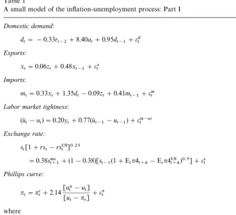
Table 1
A small model of the in#ation-unemployment process: Part I Domestic demand:
d
t"!0.33rt~2#8.40at#0.95dt~1#e$t (1) Exports:
x
t"0.06zt#0.48xt~1#ext (2)
Imports:
m
t"0.33xt#1.35dt!0.09zt#0.41mt~1#emt (3)
Labor market tightness: (u6t!u
t)"0.20yt#0.77(u6t~1!ut~1)#e(tu6~u) (4) Exchange rate:
s
t[1#rst!rsUSt ]0.25 "0.38s.#t`1#(1!0.38)[s
t~1(1#Etn4t`4!Etn4USt`4)0.5]#est (5)
Phillips curve:
n
t"nct#2.14 [uHt!u
t] [u
t!nt] #en
t (6)
where
n#t"0.73n6%t#(1!0.73!0.04!0.02)n
t~1#0.04nmt#0.02nmt~1 (7)
and
n%t"0.25[E
t~1n4t`3#Et~2n4t`2#Et~3n4t`1#Et~4n4t] (8)
19The variables were detrended using the HP "lter with a smoothing parameter of 1600; see Hodrick and Prescott (1981).
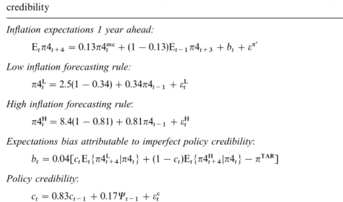
Table 2
A small model of the in#ation-unemployment process: Part II, in#ation expectations and policy credibility
Inyation expectations 1 year ahead:
E
tn4t`4"0.13n4.#t #(1!0.13)Et~1n4t`3#bt#en% (9) Low inyation forecasting rule:
n4tL"2.5(1!0.34)#0.34n4
t~1#eLt (10)
High inyation forecasting rule:
n4tH"8.4(1!0.81)#0.81n4
t~1#eHt (11)
Expectations bias attributable to imperfect policy credibility:
b
t"0.04[ctEtMn4Lt`4Dn4tN#(1!ct)EtMn4Ht`4Dn4tN!nTAR] (12) Policy credibility:
c
t"0.83ct~1#0.17Wt~1#et# (13a)
where
n
t" [eHt]2
[eHt]2#[eLt]2 (13b)
20The speci"cation explicitly treatsu!u6 as a zero mean process.
positively on a relevant measure of national wealth (a)}namely, the stock of net claims on the rest of the world (as a percent of GDP). Exports (x) exhibit a substantial degree of persistence (a coe$cient of 0.48 on the lagged dependent variable) and also depend importantly on the real exchange rate (z, an increase in which represents a real depreciation). Imports (m) likewise exhibit substantial persistence and depend in a conventional manner on domestic demand, exports, and the real exchange rate. Together, the equations for detrended domestic demand, exports, and imports describe the behavior of aggregate output relative to trend, which is used as a measure of the output gap (y, de"ned as actual output minus potential output). An important property of these equations is that there are signi"cant lags between changes in real monetary conditions
21The appropriate interest factor corresponds to one plus the per-annum interest rate di!erential expressed as a quarterly rate.
22Adjustment for the expected in#ation di!erential is a necessary condition for ensuring that the behavior of the real exchange rate is independent of the target rate of in#ation.
23See Isard (1995). Although we do not investigate the issue in this paper, we have the impression that the choice between full model consistency and a backward- and forward-looking components speci"cation of the expected future spot rate can make a considerable di!erence in using stochastic simulations to evaluate policy rules when the shocks that drive the simulations are drawn from distributions that re#ect the variances of estimated residuals for the historical period over which the model is estimated.
24As described in Appendix A, the Phillips curve is combined with an equation that describes a time-varying DNAIRU to provide a nonlinear estimation problem that can be solved using the Kalman"lter technique. Kuttner (1991, 1992, 1994) has applied this idea to measuring potential output.
25Econometric tests generally do not have su$cient power to reject either the hypopthesis that the Phillips curve is linear or the hypothesis that the Phillips curve is convex. For discussions of potential pitfalls associated with conventional tests for asymmetries in the Phillips curve, see Clark et al. (1996) and Laxton et al. (1999).
"ring costs, adjust labor inputs slowly in response to changes in the demand for their products.
In the exchange rate equation, the left-hand side variable represents the one-period forward exchange rate, which, under covered interest parity, equals the prevailing spot exchange rate appropriately adjusted for the interest rate di!erential.21The right-hand side of the equation is a standard backward- and forward-looking components model of the expected future spot exchange rate (s%t`
1), wheres.#t`1 represents the model-consistent solution and the
backward-looking component is simply the lagged spot rate adjusted for the expected in#ation di!erential.22 The measures of in#ation expectations are based on surveys of the rates of in#ation expected in Australia and the United States over the year ahead. We use the notationn4 to refer to in#ation over four quarters andnto refer to annualized rates of in#ation over one quarter; E
tn4t`1 is the
public's expectation in quartertof the rate of in#ation over the year through quarter t#4. In estimating Eq. (5), Callen and Laxton (1998) found a large weight on the backward-looking component, consistent with other evidence that high proportions of the short-run behavior of exchange rates (and other asset prices) cannot be explained by fundamentals, but rather are conditioned by the recent behavior of exchange rates (or other asset prices).23
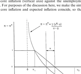
Fig. 3. The convex Phillips curve.
26In Eq. (6) the estimated value ofcis 2.14. The estimation and stochastic simulations are based on the assumption that/
t"max[0,uHt!4], and it turns out thatuHt is always strictly greater than 4 in the actual and hypothetical data we address.
27The data are based on monthly surveys of 1200 randomly selected adults. Our time series was constructed by averaging the median responses over the three months of each quarter.
28The methodology employed to develop the historical data foruHandu6involves using a Kalman "lter to solve a system of equations that includes two Phillips curves and an unemployment equation; see Callen and Laxton (1998).
viewed as an expectations-augmented Phillips curve. Consistent with the
speci-"cation in Eq. (6), the short-run Phillips curve is convex with vertical asymptote at u"/ and horizontal asymptote at n!nc"!c.26 The magnitude of
uHcorresponds to the unemployment rate at which actual in#ation and expected in#ation coincide, such that there would be no systematic pressure for in#ation to rise or fall in the absence of stochastic shocks. This corresponds to the non-accelerating-in#ation rate of unemployment in a deterministic world. We refer touHas the DNAIRU.
An important point is that the DNAIRU is not a feasible stable equilibrium in astochasticworld with a convex Phillips curve. The average rate of unemploy-ment consistent with non-accelerating-in#ation in a stochastic world, denoted byu6 and referred to as the NAIRU, must be greater than the DNAIRU when the Phillips curve is convex. This can be illustrated in Fig. 3 by assuming that actual in#ation turned out to be uniformly distributed between plus and minus one percentage point of core (or expected) in#ation, which would imply an average rate of unemployment of u6"0.5 (u
1#u2). It can easily be seen that with
a wider distribution of the actual in#ation rate around core in#ation, the average rate of unemployment would be even greater. The fact that the di! er-ence between the NAIRU and DNAIRU } and hence the average rate of unemployment }depends, in a nonlinear world, on the degree to which the authorities succeed in mitigating the variance of in#ation has important implica-tions for monetary policy, as discussed below.
29The model variants without endogenous credibility are described in Section 4 below.
2.3. Inyation expectations and policy credibility
Table 2 presents the equations that describe the behavior of in#ation expectations with endogenous policy credibility.29 The top equation focuses on explaining survey measures of in#ation expectations. As noted above, a four-quarter average of these survey measures was assumed in specifying the Phillips curve relation described in Table 1, and the simulation ex-periments described below use forecasts from Eq. (9) as hypothetical survey measures of the public's in#ation expectations. The "rst two terms in the equation are intended to represent a weighted average of a forward-looking model-consistent in#ation measure and the one-quarter lag of the survey measure of in#ation expectations. For purposes of this paper, the former measure is derived from a proxy for the model}namely, as the"tted values of an auxiliary equation that predicts observed in#ation over the year ahead using four lagged values each of the unemployment rate, a long-term interest rate, the survey measure of in#ation expectations, and the in#ation rate. The third term in Eq. (9) is intended to capture the expectations bias (b) attributable to imperfect policy credibility.
30The model for the high-in#ation state is based on work by Tarditi (1996); see the discussion in Callen and Laxton (1998). Note also that the 8.4% steady-state in#ation rate used in the high in#ation forecasting rule corresponds roughly to the average rate of in#ation in Australia during the 1980s (recall Fig. 2).
31The measures ofeHandeLare constructed by substituting the realized in#ation outcomes into the left-hand-sides of Eqs. (10) and (11), respectively. Such measures correspond to the ex-post errors associated with interpreting the realized in#ation outcomes as ex ante forecasts of in#ation under each scenario.
32Flood and Garber (1983) presented an early model of stochastic switching in policy regimes, and Hamilton (1988,1989) also contributed importantly to catalyzing the use of regime-switching models. See Laxton et al. (1994) for an application to the analysis of learning and endogenous monetary policy credibility in Canada; see Kaminsky and Leiderman (1998) for an application to developing countries.
33In a more sophisticated model of learning, the measures ofeHandeLwould be adjusted for the public's estimates of the authorities`control errors. However, the development of such a learning model is beyond the scope of this paper, which simply aims to illustrate that endogenous policy credibility is a relevant consideration in the design of monetary policy rules.
rate expected under the high-in#ation scenario can be described by Eq. (11).30
Eq. (12) de"nes the measure of expectations bias, where the terms in square brackets measure the discrepancy between the in#ation target (nTAR) and a weighted average of the in#ation forecasts under the two scenarios. As re#ected in Eq. (13a), the weight on the low-in#ation scenario (c) is treated as a time-varying parameter that exhibits a high degree of persistence (as implied by the model estimates), but changes from period to period by an amount that re#ects the extent to which in#ation outcomes are more consistent with the low in#ation scenario than with the high in#ation scenario. The termt, as de"ned in Eq. (13b), provides our measure of the extent to which in#ation outcomes are consistent with the low-in#ation scenario.31Note that if in#ation outcomes are repeatedly completely consistent with the low-in#ation scenario, eL"0 and
t"1, so cconverges to unity. Likewise, if in#ation outcomes are repeatedly completely consistent with the high in#ation scenario,eH"0,t"0, andc con-verges to zero.
The above two-scenario paradigm bears a resemblance to a two-state re-gime-switching model with time-varying transition probabilities.32 Note that the in#ation target coincides with the steady-state outcome under the low in#ation scenario (i.e., the model is estimated and simulated withnTAR"2.5); that c
t can be interpreted as the subjective probability attached to the low in#ation state; and that in the limiting case ofc
5"1, long-run in#ation
expecta-tions coincide with the in#ation target. Based on the latter two properties, we regard c
5 as a measure of the stock of credibility at time t. Although the
Fig. 4. Historical perspectives on policy credibility.
behaving in a stable manner (not subject to multiple equilibria) and converging to zero as cconverges to one. Furthermore, the estimated behavior ofc
t and
34The assumption of boundedness seems conceptually appropriate. However, the results we report in this paper are based on simulations that are all initialized with the DNAIRU at 7.0, and in which the DNAIRU rarely if ever hits its#oor or ceiling.
35Callen and Laxton (1998) describe the methodology employed to develop the historical estimates of the DNAIRU and NAIRU.
36From technical and strategic perspectives, giving the authorities knowledge of the period-t
in#ation rate reduces the incidence of unstable stochastic simulations for the Taylor rule cases and appears to act in the direction of understating the extent to which IFB rules dominate Taylor rules in our simulation experiments.
3. The stochastic simulation framework and selected policy rules
3.1. The Monte Carlo experiments
The assumptions underlying our Monte Carlo experiments are as follows:
1. The &true model' of macroeconomic behavior consists of the equations in Tables 1 and 2 (with di!erent versions of Eqs. (6) and (9) under di!erent model variants, as described below), together with the monetary policy rule and a process (described in Appendix A) that generates the evolution of the DNAIRU and NAIRU over time.
2. The DNAIRU follows a bounded random walk34 with #oor at 4% and ceiling at 10%. Conditional on not hitting either bound, the DNAIRU changes from one quarter to the next by a random amount drawn from a normal distribution with mean zero and standard deviation corresponding to that of the distribution of estimated DNAIRUs during the historical sample period;35for cases in which the DNAIRU could not change by the full amount of the random draw without moving below 4% or above 10%, the DNAIRU moves to its #oor or ceiling, respectively.
3. In each period t, the monetary authorities update their estimate of the DNAIRU and set the period-t interest rate based on an information set
X
t that includes: the complete speci"cation of the true model except for the process that generates the DNAIRU and NAIRU (i.e., complete information about Eqs. (1)}(3) and (5)}(14)); the history of all observable variables (includ-ing the survey measures of in#ation expectations) through periodt!1, as
well as the in#ation rate for periodt; and the probability distributions (but not the realizations) of the shocks for periodt and all future periods. This implicitly assumes that the in#ation rate is the"rst relevant period-tstatistic that becomes known to the authorities, and that the period-tinterest rate is set immediately following the arrival of information about the period-t
37The procedure that the authorities are assumed to use to update their estimates of the DNAIRU and NAIRU is described in Appendix A.
38A value of 50 quarters is su$ciently long to insure that errors in the terminal conditions will not induce errors in the variables of interest. Under in#ation targeting, the price level has a unit root, and the procedure for period-to-period updating of the authorities'forecasts also involves period-to-period updating of the terminal conditions.
generate the DNAIRU and NAIRU, they update their estimates of these parameters each period on the basis of their information about the structure of the model and the history of unemployment and in#ation.37
4. The exogenous shocks are drawn from independent normal distributions with zero means and standard deviations that re#ect the unexplained vari-ances of the dependent variables during the historical periods over which the equations were estimated.
5. The authorities use a prespeci"ed policy rule, along with the assumption that the realizations of random shocks beyond periodt will coincide with their expected values of zero, to determine the interest rate setting for period
t and to generate forecasts of the complete future timepaths of all the macroeconomic variables in the model, including interest rates and the DNAIRU.
Given these assumptions, for each candidate policy rule we simulate a hypothetical path of the economy over a horizon of 100 quarters. Starting in period t, the monetary authorities observe data through period t!1, update their forecasts for all variables through the end of a 50-quarter horizon,38 including their forecasts for the period-t values of the variables that enter the policy rule (with perfect foresight or advanced knowledge of the period-tin#ation rate), and determine the period-tinterest rate setting. After the forecasts are generated and the interest rate is set, the shocks for period
t are drawn randomly (but consistently with the prespeci"ed probability distributions) and the period-tvalues of relevant variables are determined from the true model. The determination of the period-t solution is based on the assumptions that the (expected) future path of the real interest rate coincides with the authorities'forecast, and that the NAIRU follows the process described by the true model. After the period-t solution is added to the hypothetical history of the economy, the authorities generate updated forecasts (including updated estimates of the NAIRU) and set the interest rate for periodt#1, and so forth.
39For the model variants with endogenous policy credibility, a few draws of the random shocks led to explosive simulations under rule calibrations that placed relatively high weights on the unemployment gap}speci"cally, the (a,c)"(0.5, 1) calibrations; see below. We actually performed somewhat more than 100 sets of simulations and then discarded the results for the draws in which convergence failure was experienced under any one of the rule calibrations.
40For example, Rudebusch and Svensson (1999). Somewhat analogously, Levin et al. (1999) focus on minimizing the"rst two terms of (14) subject to an upper bound on the third term.
41Faust and Svensson (1999) focus on a similar loss function withb'0 in analyzing the pros and cons of central bank transparancy.
42The settingl"0.5 corresponds to the base-case value used by Rudebusch and Svensson (1999).
43The simulations set/
t"uHt!4, so the convex term in the unemployment rate in Eq. (6) can be expressed as 2.14F(g), whereg"uH!u. The linear approximation in Eq. (6a) replacesF(g) with [F@(0)](uH!u)"(2.14/4)(uH!u)"0.535(uH!u).
using the same 100 sequences of randomly drawn shocks.39 For purposes of evaluating the relative attractiveness of the di!erent rules and rule calibrations, we de"ne the loss function
¸
t"(nt!nTAR)2#h[ut!(uHt!b)]2#l(rst!rst~1)2 (14)
whereh,b, andlare parameters anduHt is the DNAIRU (deterministic NAIRU). For b"0 this corresponds to the speci"cation that has been used in other recent simulation studies of monetary policy rules.40 More generally, it also allows us, somewhat in the spirit of Barro and Gordon (1983a,b) and Rogo!
(1985), to consider cases in which the authorities' preferences with regard to unemployment are not symmetric around the DNAIRU but center on an unemployment rate below the DNAIRU (i.e., cases withb'0).41For each of the alternative rules and rule calibrations we compare the simulated sample means and standard deviations of the in#ation rate and the unemployment rate and calculate, as a summary statistic, the sum of the 10,000 observations on
¸
t for the base-case parameter settings (b,h,t)"(1, 1, 0.5).42
3.2. The modelvariants
The relative performance of the policy rules were evaluated within each of six variants of the basic model. In the"rst three variants, the convex Phillips curve (Eq. (6) in Table 1) was replaced with the linear approximation43
n
t"nct#0.535(utH!ut)#ent. (6a) For the"rst of these cases, as well as the"rst case with a convex Phillips curve, we assume that the public forms its in#ation expectations in a backward-looking manner; thus, we replace Eq. (9) with
E
44Forward-looking IFB rules have been used for almost a decade at the Bank of Canada to solve nonlinear macroeconomic models designed for policy analysis. With the development of more robust and e$cient solution methods, these rules are now starting to be used in other policymaking institutions. See Armstrong and others (1998) and Julliard and others (1998) for a discussion of the algorithms that can be used to solve these types of models.
45On IFB rules see Amano et al. (1999) and Batini and Haldane (1999).
Under the second case for each class of Phillips curves, it is assumed that the public forms its in#ation expectations in a forward-looking manner but treats policy credibility as exogenous. For these cases the simulations retain Eq. (9) but set b
t"0 for all t. The third model variant for each class of Phillips curve is forward-looking with endogenous policy credibility.
3.3. The policy rules
For each of the six model variants we used our stochastic simulation experi-ments to evaluate macroeconomic performance under two forms of policy rules: Taylor rules and analogous in#ation forecast based (IFB) rules.44 Part of the motivation for focusing on these linear forms of policy rules is pragmatic; particularly in the nonlinear variants of our model, the task of deriving the optimal functional form would be horrendous. In addition, simple classes of rules are transparent and relatively appealing to policymakers, Taylor rules have been popular in the literature since the early 1990s, and IFB rules have been shown to deliver reasonable economic performances over a wide range of disturbances.45 It may be noted that linear IFB rules, by focusing on the deviation from target of the authorities' in#ation forecast, have the appealing feature (in comparison with Taylor rules) of taking account of any nonlinearities in the macroeconomic model insofar as the in#ation forecast re#ects the struc-ture of the model.
The two classes of rules were speci"ed in the general forms:
r
t"rH#E3tMa(nt!nTAR)#c(u6t!ut)DXtN, (15) and
r
t"rH#E3tMa(nt`3!nTAR)#c(u6t!ut)DXtN, (16) where
r
t"rst!E3tMEtn4t`4DXtN. (17) Herers
t is the nominal interest rate setting at timet;rtis the concept of the real interest rate on which aggregate demand depends; E
46Taylor's (1993) version of the Taylor rule used a backward looking measure of in#ation expectations to measure the real interest rate.
47We have not undertaken an extensive search for the optimal in#ation forecast horizon. It may be noted that three quarters is roughly half the time that is generally believed to be required for interest rates to have their full e!ects on the economy.
48See Isard et al. (1999) for stability analysis of conventional Taylor rules in linear and nonlinear variants of a closed-economy model of the U.S. economy. In that study, simulations with conven-tional Taylor rules in the nonlinear model variants with forward-looking expectations generated explosive behavior under most drawings of the random shocks.
expectations at timetof the in#ation rate over the year ahead;rHis a constant corresponding to the equilibrium real interest rate in a deterministic world under the prespeci"ed initial conditions of the economy;nTARdenotes the target rate of in#ation; E3tMDX
tNdenotes a model-consistent forecast at timetbased on the authorities information setX
t, which includes information about the model along with the observed values of the in#ation rate through period t and all other economic variables through quartert!1;ntandu
trepresent the rates of in#ation and unemployment; andu6
t is the authorities'estimate of the NAIRU based on observed data through periodt!1 (see Appendix A). The bracketed
terms in Eqs. (15) and (16) are relatively traditional components of policy reaction functions discussed in the literature, corresponding to the deviation of in#ation (or the authorities'in#ation forecast) from target and the deviation of the unemployment rate from the NAIRU.46 Experimentation suggested that specifying the second class of rules in terms of an in#ation forecast that looks ahead three quarters was capable of producing reasonable macroeconomic stability.47
Note that the policy reaction functions are speci"ed in the form of rules for real interest rate adjustment. Although monetary policy operates by setting the nominal interest rate, in our model (and most others) the extent to which monetary policy adjustment stimulates or restrains aggregate demand depends on the change in the real interest rate. It would thus make no sense to propose that policy be guided by a nominal interest rate rule that could not be explicitly translated into an economically reasonable rule for the real interest rate on which aggregate demand depends.
Note also that in four of the six model variants, the Taylor rule de"ned by Eqs. (15) and (17) embodies a forward-looking measure of the real interest rate. By contrast, the conventional form of the Taylor rule embodies a backward-looking measure of the real interest rate, as in the two model variants that impose condition (9a). In general, a conventional completely-backward-looking Taylor rule performs worse than the Taylor rule de"ned by Eqs. (15) and (17).48
49See Isard and Laxton (1999). We also experimented with a third calibration of the Taylor rule, namely (a,c)"(0.5, 2), corresponding to a suggestion in Taylor (1999). Our results suggested that moving from (0.5, 1) to (0.5, 2) tends to worsen macroeconomic performance under conditions of NAIRU uncertainty and endogenous policy credibility. Consistently, the results reported below suggest that performance under a Taylor rule can be improved by moving from (0.5, 1) to (2, 1).
50It may be noted that the sample means and standard deviations of the DNAIRU are identical for all combinations of model variants and policy rules, re#ecting the fact that in each case the stochastic simulations are based on identical initial positions and sequences of random shocks.
51Other papers that have employed stochastic simulations to evaluate the performances of monetary policy rules have focused almost exclusively on linear models and have often summarized the relative performances of di!erent rules by plotting the associated standard deviations of unemployment and in#ation on a two-dimensional graph.
The "rst calibration, (a,c)"(0.5, 1), corresponds roughly to the weights originally suggested for the U.S. case by Taylor (1993), after adjustingcfor the fact that Taylor speci"es his rule in terms of the output gap rather than the unemployment gap, and that the unemployment gap tends to vary about half as much over business cycles as the output gap. The second parameter setting, (a,c)"(2, 1), is based on a calibration of the in#ation forecast based (IFB) rule that we found to perform relatively well in another study.49We later report, and discuss the limited relevance of, simulation results for the (approximately) optimal Taylor rule calibrations for two of the model variants.
4. Simulation results
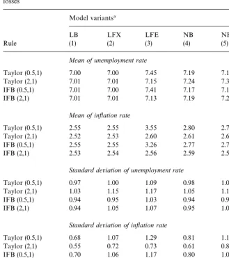
Table 3 reports simulation results for the means and standard deviations of unemployment and in#ation, along with the cumulative welfare losses, under each of the six di!erent model variants and four di!erent policy rules.50For the linear model variants without endogenous policy credibility (columns 1 and 2), the choice of monetary policy rule (after conditioning on a prespeci"ed in#ation target) has almost no e!ects on the mean rates of in#ation and unemployment
Table 3
Simulated means and standard deviations of unemployment and in#ation, and cumulative welfare losses
Model variants!
LB LFX LFE NB NFX NFE
Rule (1) (2) (3) (4) (5) (6)
Mean of unemployment rate
Taylor (0.5,1) 7.00 7.00 7.45 7.19 7.19 7.91
Taylor (2,1) 7.01 7.01 7.15 7.24 7.32 7.55
IFB (0.5,1) 7.01 7.00 7.41 7.17 7.16 7.84
IFB (2,1) 7.01 7.01 7.13 7.19 7.25 7.45
Mean of inyation rate
Taylor (0.5,1) 2.55 2.55 3.55 2.80 2.79 4.27
Taylor (2,1) 2.52 2.53 2.60 2.61 2.64 2.73
IFB (0.5,1) 2.55 2.55 3.26 2.77 2.73 3.83
IFB (2,1) 2.53 2.54 2.56 2.59 2.59 2.64
Standard deviation of unemployment rate
Taylor (0.5,1) 0.97 1.00 1.09 0.98 1.00 1.29
Taylor (2,1) 1.03 1.15 1.17 1.05 1.18 1.22
IFB (0.5,1) 0.94 0.95 1.03 0.94 0.95 1.21
IFB (2,1) 0.94 1.05 1.07 0.95 1.05 1.11
Standard deviation of inyation rate
Taylor (0.5,1) 0.68 1.07 1.29 0.81 1.14 1.63
Taylor (2,1) 0.55 0.72 0.73 0.61 0.84 0.81
IFB (0.5,1) 0.70 1.06 1.17 0.80 1.09 1.39
IFB (2,1) 0.57 0.71 0.71 0.62 0.75 0.74
Cumulative welfare loss"
Taylor (0.5,1) 10.35 11.74 20.54 11.90 13.15 30.44
Taylor (2,1) 10.83 12.06 12.50 11.41 13.33 14.04
IFB (0.5,1) 10.20 11.44 17.34 11.56 12.46 25.02
IFB (2,1) 10.14 11.19 11.39 10.52 11.68 12.37
!The LB, LFX, and LFE variants have linear Phillips curves; NB, NFX, NFE have nonlinear Phillips curves. The LB, NB variants have backward looking expectations; LFX, NFX have looking expectations but treat policy credibility as exogeneous; LFE, NFE have forward-looking expectations and treat policy credibility as endogenous.
"Corresponds to the (normalized) sum of the 10,000 observations for¸
52Taylor's (1999) suggestion was that a calibration of (0.5, 1) would outperform (0.5, 0.5, 5) in a rule speci"cation analogous to Eq. (15) but with the output gap in place of the unemployment gap. As noted earlier, based on a rough estimate that the unemployment gap tends to vary about half as widely as the output gap over the business cycle, we view a weight of unity on the unemployment gap as broadly comparable to a weight of 0.5 on the output gap.
53See also Smets (1999) and Drew et al. (1999).
54This result does not necessarily imply that estimates of the unemployment gap are too imprecise to inform monetary policy in a useful way, even though the authorities'estimates of the unemployment gap may often be incorrect in sign as well as in magnitude. In particular, in simulations not reported in this paper, we have shown that IFB rules that place no weight on the unemployment gap are dominated by other calibrations.
For the two cases of convex Phillips curves without endogenous policy credibility (columns 4 and 5), the IFB rules produce slightly lower means for both unemployment and in#ation, as well as lower standard deviations for the case with forward-looking expectations, in comparison with the corresponding Taylor rules. Consistently, the IFB rules generate somewhat lower values for the summary measure of the cumulative welfare loss. With regard to the two alternative calibrations, we again "nd a hardly surprising result; within each class of reaction functions, the rule with relatively stronger reaction to the unemployment gap (i.e., the (0.5, 1) calibration) generates a lower mean for the unemployment rate and a higher average in#ation rate.
The results are qualitatively di!erent and quantitatively more striking in the cases with endogenous policy credibility. For the case with a linear Phillips curve and endogenous credibility (column 3), the sensitivity of performance to the choice of weights is signi"cantly greater than in the linear cases without endogenous credibility, and the means ofbothunemployment and in#ation are lower under the (2, 1) calibrations, which are more responsive to deviations from equilibrium in an absolute sense but relatively less responsive to the unemploy-ment gap. This result suggests that in seeking to improve upon the policy rule calibration that Taylor (1993) suggested for the United States, a calibration that gives relatively more weight to the output/unemployment gap, as discussed by Taylor (1999) may be inferior to a rule that places relatively more weight on the deviation of in#ation from target.52 In this context, it seems important to recognize that in a world with considerable uncertainty about the NAIRU, policymakers are bound to make signi"cant errors in estimating the unemploy-ment gap, and such errors are likely to be positively autocorrelated.53Given that the Phillips curve tends to transmit systematic errors in estimating the unemployment gap into changes in the in#ation rate, the greater the uncertainty that surrounds estimates of the unemployment gap, the stronger should be the policy reaction to in#ation relative to unemployment, other things equal.54
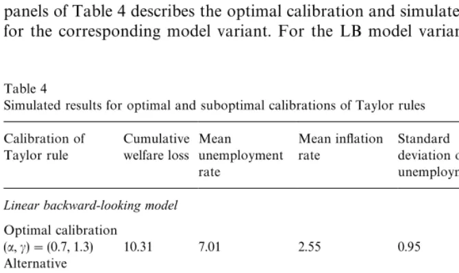
Table 4
Simulated results for optimal and suboptimal calibrations of Taylor rules Calibration of Nonlinear forward-looking model with endogenous policy credibility
Optimal calibration
(a,c)"(1.8, 0.8) 13.72 7.41 2.67 1.21 0.82 Alternative
calibration
(a,c)"(0.7, 1.3) 25.27 7.86 3.86 1.24 1.37
a nonlinear Phillips curve (column 6). Consider, in particular, the di!erence between the (0.5, 1) Taylor rule, which reacts relatively weakly to in#ation, and only after changes in the in#ation rate are observed, and the (2, 1) IFB rule, which reacts relatively strongly to the in#ation forecast. The mean unemploy-ment rate is nearly 1/2 of a percentage point lower in the latter case, while the mean in#ation rate is more than 1 1/2 percentage points lower. For the case with endogenous credibility and a linear Phillips curve (column 3), the choice be-tween the same two rules makes a di!erence of roughly 1/3 of a percentage point for the average unemployment rate and 1 percentage point for the average in#ation rate.
We draw two inferences from the results in Table 3. First, the (0.5, 1) calib-ration suggested by Taylor (1993) is dominated across a range of model variants by a calibration that responds more aggressively to deviations from target, and with a relatively greater weight on in#ation than on unemployment. Second, forward-looking IFB rules tend to dominate backward-looking Taylor rules.
calibration reacts with a weight of 0.7 to deviations of in#ation from target and 1.3 to the unemployment gap, generating a policy loss of 10.31. This calibration corresponds fairly closely to the two calibrations suggested by Taylor (1993,1999)}namely, (a,c)"(0.5, 1) and (a,c)"(0.5, 2)}and achieves a degree of macroeconomic stability only very slightly better than the (0.5, 1) calibration, which generates a policy loss of 10.35 (recall Table 3). For the NFE model variant the optimal calibration reacts with a weight of 1.8 to the deviation of in#ation from target and 0.8 to the unemployment gap, generating a policy loss of 13.72 }slightly lower than that generated by the (a,c)"(2, 1) calibration
shown in Table 3.
The bottom line in each panel of Table 4 describes the macroeconomic performance that results from following the optimal Taylor rule calibration for the other model variant. Note, "rst, that the optimal calibration for the LB variant performs very poorly in the NFE variant and, second, that relative to the optimal outcomes for each model variant, the optimal calibration for the LB variant performs much more poorly in the NFE variant than the optimal calibration for the NFE variant performs in the LB variant. As can be seen in the bottom line of the table, adopting the optimal LB calibration in the NFE model variant has the stag#ationary e!ect of raising both the average unemployment rate and the average in#ation rate relative to the outcomes for the optimal NFE calibration.
Such results illustrate that knowledge of the optimal policy-rule calibration associated with a speci"c macro model has little relevance for policymaking in the absence of a strong presumption that the model is true; indeed, the optimal calibration for a speci"c hypothetical model can perform very poorly in a some-what di!erent model variant. This is the type of "nding that has motivated McCallum (1988) and Levin et al. (1999) to search for rules and rule calibrations that perform well across a variety of plausible macro models.
The results also challenge the traditional practice of relying heavily on linear macro models for evaluating policy rules and rule calibrations. Although Table 4 presents a very limited set of results, it provides a basis for the conjecture that rules and rule calibrations that perform well in nonlinear models with forward-looking expectations are much more robust than rules and rule calibrations that perform well in linear models with backward-looking expectations. As an inference speci"c to the class of Taylor rules that this paper analyzes, our results suggest that, in general, policymakers should react more aggressively to devi-ations from in#ation/unemployment targets than has been inferred from simula-tion analysis based on linear macro models.
55See, for example, Amano et al. (1999) and Batini and Haldane (1999) for studies that have in#uenced thinking at the Bank of Canada and Bank of England, respectively. See Kohn (1999) for perspectives on how information about the implications of monetary rules helps structure thinking by some members of the U.S. Federal Open Market Committee.
56See, for example, McCallum (1988) and Levin et al. (1999).
contrast with Taylor's (1993, 1999) suggestions, this result recognizes that when policymakers make relatively large and serially correlated errors in estimating unemployment gaps, it can be costly in a nonlinear world to react very strongly to their estimates of unemployment gaps, even when they attach relatively high policy losses to unemployment.
5. Conclusions
The economics profession has taken signi"cant strides in recent years in using simple macroeconomic models to analyze the relative performances of di!erent hypothetical policy rules. Although many economists and policymakers recog-nize that mechanical adherence to a simple policy rule would be a recipe for disaster, such analysis has been helpful in advancing the conceptual framework for formulating in#ation targeting strategies, and information derived from simple policy rules is regularly used by some central bankers to help structure thinking about the settings of monetary policy instruments.55At the same time, contributors to the recent research on monetary policy rules have emphasized concerns about the validity of inferences drawn from speci"c macro models and have made e!orts to explore the robustness of their conclusions.56
This paper has been motivated by the observation that in their search for robust policy rules, economists have not yet adequately explored how their proposed rules perform in models with endogenous policy credibility, NAIRU uncertainty, and convex Phillips curves. Most (if not all) central bank governors in industrial countries regard endogenous policy credibility and NAIRU uncer-tainty as fundamental characteristics of the worlds in which monetary policy must be conducted, and we regard convex Phillips curves as another important reduced-form feature of the real world.
57As noted earlier, in simulation analysis of a closed-economy model of the United States, Isard et al. (1999) found that in nonlinear model variants with forward-looking expectations, conventional Taylor rules led to explosive behavior for most drawings of random shocks.
models, moreover, we are asked to believe that monetary policy has no" rst-order e!ects on welfare in the sense that, for a given target in#ation rate, the choice of policy rule has no in#uence on the average rates of unemployment or in#ation that economies experience over time. Because such studies do not adequately address the commonly-observed phenomenon of prolonged periods of bias between in#ation expectations and in#ation outcomes, which presum-ably re#ects the nature of monetary policy, their evaluations of policy rules abstract from an important feature of the monetary policy transmission mechanism.
By contrast, the analysis in this paper has focused on the implications of endogenous policy credibility. Our comparisons of how rules perform in several di!erent model variants suggest that the introduction of endogenous credibility leads to some qualitatively di!erent and quantitatively more striking perspect-ives on the choice between the di!erent calibrations of Taylor rules and IFB rules, and that these perspectives are reinforced by the introduction of convex Phillips curves. More speci"cally, our simulation results suggest that in a world that embodies the long-run natural rate hypothesis, and in which credibility and in#ation expectations respond endogenously to the track record of the authori-ties in delivering low in#ation, with credibility more easily lost than regained, forward-looking IFB rules tend to have a signi"cant advantage over Taylor rules. Moreover, for a given target rate of in#ation, the choice between di!erent calibrations of the reaction parameters has signi"cant implications for the means of the unemployment rate and the in#ation rate, as well as for the variances of unemployment and in#ation. In this connection, the (0.5, 1) calib-ration } which broadly corresponds to the parameter values suggested by Taylor (1993) for the U.S. economy}is signi"cantly outperformed by a calib-ration that reacts more forcefully to deviations from targets, and with relatively stronger reactions to deviations from the in#ation target than to unemployment gaps.
It should be emphasized that the Taylor rule speci"cation we have analyzed in this paper essentially assumes that the policymaker adjusts a model-consistent measure of the real interest rate in reaction to the most recent observations of in#ation and unemployment. For four of our six model variants this speci" ca-tion gives the Taylor rule signi"cantly stronger stabilizing properties than the conventional speci"cation, which embodies a backward-looking measure of the real interest rate.57
58This is especially the case for the conventional form of the Taylor rule, which embodies a backward-looking measure of the real interest rate and reacts to a backward-looking measure of in#ation.
that backward-looking Taylor rules perform well in linear macro models with exogenous policy credibility, this"nding begins to break down with the intro-duction of nonlinearities, such as those associated with endogenous credibility, convex Phillips curves,#oors on nominal interest rates, asymmetric hysteresis in labor markets, and so forth. It may also be noted that}for the speci"c model variants analyzed in this paper}simple linear policy rules that embody model-consistent in#ation measures of real interest rates and react to model-consistent in#ation forecasts appear to be reasonably successful in stabilizing the economy. The conclusions of simulation studies inevitably depend on the particular models that are analyzed as well as on the parameterization of the policy loss function. For that reason we have focused on six di!erent model variants and looked through the summary loss statistics by reporting the means and standard deviations of in#ation and unemployment.
Intuitively, the following line of argument provides strong reason to suspect that our conclusions about the relative stabilizing properties of Taylor rules and IFB rules generalize to other plausible nonlinear models and loss function parameterizations. First, in nonlinear models with forward-looking agents, success in preventing an acceleration of in#ation generally hinges on the e! ec-tiveness of the monetary authorities in avoiding prolonged states of excess demand. Second, in most macro models adjustments in the nominal interest rate are transmitted to aggregate demand primarily through the real interest rate. Third, in reality monetary policymakers confront considerable uncertainty about the behavior of the economy, and economists tend to make serially correlated errors in estimating output and unemployment gaps, so even the best informed policymakers occasionally come to realize that they had been mis-guaging the strength of the economy in the recent past, and that their policy errors have led to a state of signi"cant excess demand. And"nally, when an economy is experiencing signi"cant excess demand, the nominal interest rate adjustments that would be dictated by a backward-looking Taylor rule may be insu$cient to raise the level of the real interest rate that is perceived by forward-looking market participants, and might therefore allow excess demand to continue to strengthen, accompanied by a continuing upward spiral in market participants'in#ation expectations.58
Appendix A. An updating procedure for estimating the NAIRU
knowledge of the structure of the model and the histories of both the unemploy-ment rate and the in#ation rate. To investigate the implications of uncertainty about the NAIRU, it is assumed that the authorities know the true structure of the Phillips curve
Inferences about these unobservable variables can be derived from informa-tion about the structure of the Phillips curve as well as historical informainforma-tion about movements in n, n#, and u. However, it is well known that because of signi"cant measurement error in the Phillips curve relationship (ent in Eq. (A.1)), there can be signi"cant errors in the estimates ofuHt derived directly from the Phillips curve. For this reason it has been common for researchers in policy making institutions to also base their estimates of the NAIRU on trend move-ments in unemployment rates.
The analysis in this paper is based on an updating process for the DNAIRU (and the NAIRU) that takes account of historical information about both unemployment and in#ation and can be formulated as an explicit Kalman
"ltering problem in which the monetary authorities are assumed to gradually learn about shifts in the underlying DNAIRU. We assume that the authorities operate under the assumption that the DNAIRU is subjected to permanent shocks, or that the change in the DNAIRU follows a random walk according to
uHt"uHt
~1#eutH, (A.2)
whereeuH
t is distributed as N(0,puH), withpuHmeasuring the degree of volatility in
the underlying DNAIRU. In addition, the monetary authorities are assumed to know that for a given policy rule, there will be a constant di!erence (a) between the NAIRU and DNAIRU.
a"u6
t!uHt. (A.3)
Finally, the monetary authorities are assumed to know that the business cycle component of unemployment,eut, is a stationary process with a"xed mean of zero.
u
59In the true model we assume that the DNAIRU process is a bounded random walk that ranges between 4 and 10. However, for the purpose of updating the uH and u6 estimates we make a simplifying assumption that the monetary authorities are not able to observe these bounds and therefore act as if the DNAIRU process is unbounded. An alternative would be to relax this assumption, in which case the monetary authorities would always forecast the DNAIRU to gradually return back to a"xed steady state value. This would somewhat increase the complexity of our programming problem but probably would not add much additional insight.
as the &true' degree of volatility in the underlying DNAIRU estimates. This results in an orderly updating process for the DNAIRU and NAIRU, where the monetary authorities make mistakes estimating the NAIRU and gradually improve their historical estimates over time as new data are released on in#ation and unemployment developments.
The solution technique in the Monte Carlo experiments involves the follow-ing process.
The solution at the beginning of periodtprovides estimates of the histories of the DNAIRU and NAIRU through period t!1, along with forecasts of the
DNAIRU and NAIRU through a terminal simulation horizon¹. The forecasts
are based on the assumption that realizations of all future shocks coincide with the zero means of the probability distributions of the shocks. Thus, in periodt, the DNAIRU and NAIRU are forecast to remain unchanged at their estimated periodtvalues.59
In the context of the stochastic simulations, after the Kalman"ltering prob-lem has been solved at the beginning of periodt, hypothetical realizations of the periodtshocks are randomly drawn using Monte Carlo techniques, and the true model is then solved for the periodtvariables. Then the process is repeated, as the authorities again solve the Kalman"ltering problem using the additional period of&historical data'to update their historical estimates and forecasts of the DNAIRU and NAIRU.
References
Amano, R., Coletti, D., Macklem, T., 1999. Monetary rules when economic behavior changes. In: Hunt, B., Orr, A. (Eds.), Monetary Policy Under Uncertainty, Reserve Bank of New Zealand, Wellington, 157}200.
Armstrong, J., Black, R., Laxton, D., Rose, D., 1998. A robust method for simulating forward-looking models. Journal of Economic Dynamics and Control 22, 489}501.
Barro, R.J., Gordon, D.B., 1983a. Positive theory of monetary policy in a natural rate model. Journal of Political Economy 91, 589}610.
Barro, R.J., Gordon, D.B., 1983b. Rules, discretion, and reputation in a model of monetary policy. Journal of Monetary Economics 12, 101}121.
Bernanke, B.S., Mishkin, F.S., 1997. In#ation targeting: a new framework for monetary policy? Journal of Economic Perspectives 11, 97-116.
Callen, T., Laxton, D., 1998. A Small Macro Model of the Australian In#ation Process with Endogenous Policy Credibility. International Monetary Fund, Washington, unpublished. Clark, P., Laxton, D., 1997. Phillips curves, Phillips lines and the unemployment costs of
overheat-ing. Working Paper 97/17, International Monetary Fund, Washington, February.
Clark, P., Laxton, D., Rose, D., 1996. Asymmetry in the U.S. output-in#ation nexus: issues and evidence. IMF Sta!Papers 43, 216}250.
Debelle, G., 1997. In#ation targeting in practice. IMF Working Paper 97/35, International Monet-ary Fund, Washington, March.
Debelle, G., Laxton, D., 1997. Is the Phillips curve really a curve? Some evidence for Canada, the United Kingdom, and the United States. Sta!Papers 44, 249}282.
Debelle, G., Vickery, J., 1997. Is the Phillips curve a curve? Some evidence and implications for Australia. Economic Research Department, Reserve Bank of Australia, unpublished paper. Drew, A., Hunt, B., Scott, A., 1999. E$cient simple policy rules and the implications of uncertainty
about potential output. In: Hunt, B., Orr, A. (Eds.), Monetary Policy Under Uncertainty, Reserve Bank of New Zealand, Wellington, 73}102.
Faust, J.W., Svensson, L.E.O., 1999. Transparency and credibility: monetary policy with unobserv-able goals. Revised Draft of NBER Working Paper 6452, April.
Federal Reserve Bank of Kansas City, 1996. Achieving Price Stability: A Symposium. Kansas City, Missouri.
Fischer, S., 1996. Why are central banks pursuing long-run price stability? In: The Federal Reserve Bank of Kansas City, Achieving Price Stability: A Symposium.
Flood, R., Garber, P., 1983. A model of stochastic policy switching. Econometrica 51, 537}552. Flood, R., Isard, P., 1989. Monetary policy strategies. Sta!Papers. International Monetary Fund 37,
446}448.
Flood, R., Isard, P., 1990. Monetary policy strategies*a correction. Sta!Papers, International Monetary Fund 37, 446}448.
Freedman, C., 1996. What operating procedures should be adopted to main price stability? *practical issues. In: The Federal Reserve Bank of Kansas City, Achieving Price Stability: A Symposium.
Haldane, A.G. (Ed.), 1995. Targeting In#ation. Bank of England, London.
Hamilton, J.D., 1988. Rational-expectations econometric analysis of changes in regime * an investigation of the term structure of interest rates. Journal of Economic Dynamics and Control 12, 385}423.
Hamilton, J.D., 1989. A new approach to the economic analysis of nonstationary time series and the business cycle. Econometrica 57, 357}384.
Hodrick, R.J., Prescott, E.C., 1981. Post-war U.S. business cycles: an empirical investigation. Carnegie-Mellon Discussion Paper No. 451, Carnegie-Mellon University, Pittsburgh, May. Isard, P., 1995. Exchange Rate Economics. Cambridge University Press, Cambridge.
Isard, P., Laxton, D., 1996. Strategic choice in Phillips curve speci"cation: what if Bob Gordon is wrong? Presented at a Conference on European Unemployment: Macroeconomic Aspects, Florence, Italy.
Isard, P., Laxton, D., 1999. Monetary policy with NAIRU uncertainty and endogenous policy credibility: perspectives on policy rules and the gains from experimentation and transparancy. In: Hunt, B., Orr, A. (Eds.), Monetary Policy Under Uncertainty, Reserve Bank of New Zealand, Wellington, 33}65.