IMPLEMENTATION AND TESTING
5.1 Implementation
Backpropagation learning process with 1, 2 and 3 hidden layers have many methods, there are InitiationWeight(), Znet(), Z(), Ynet() and Y(), Unet(), U(), ∆W(), UpdateWeight(). With the same concepts and formulas, Backpropagation 2 and 3 hidden layers repeat the Znet(), Z(), Unet(), U() and ∆Weight() methods. This is done because the method contains the process of calculating values on nodes in the hidden layer.
1. public void InitiationWeight()
2. {
3. Random rand = new Random();
4. for (i=0;i<weight1.length;i++)
5. {
6. for (j=0;j<weight1[0].length;j++)
7. {
8. weight1[i][j]= (-1) + (1-(-1))*rand.nextDouble();
9. }
10. }
11. for (i=0;i<weight2.length;i++)
12. {
13. for (j=0;j<weight2[0].length;j++)
14. {
15. weight2[i][j]= (-1) + (1-(-1))*rand.nextDouble();
16. }
17. }
18.}
The InitiationWeight() method is used to initialize the initial weight using random numbers between -1 to 1 according to the formula in the Backpropagation algorithm. In line 3, the rand variable uses the Random library of import java.util.Random. Line 4-10 initiates weight on weight1, which is the weight
between input layer and hidden layer. Line 11-17 is the initiation of weight2, which is the weight between the hidden layer and the output layer. The InitiationWeight() method is executed at the start of the learning process.
19.public void Znet()
20.{
21. for(i=0;i<znet.length;i++)
22. {
23. znet[i]=0;
24. }
25. for(i=0; i<znet.length; i++)
26. {
27. for(j=0; j<input.length; j++)
28. {
29. znet[i]= znet[i]+ (weight1[j][i]*input[j]);
30. }
31. }
32.}
The Znet() method is used to calculate the value in the hidden layer nodes. Line 21-24 is the initial value of znet is 0. Line 25-31 computes each value in the hidden layer nodes by summing all entries multiplied by the weight1 that towards to each nodes in the hidden layer. The value of weight1 is derived from the Initiationweight() method which is then updated in the UpdateWeight() method.
33.public void Z()
34.{
35. for(i=0; i<znet.length; i++)
36. {
37. z[i]= 1/(1+Math.exp(-znet[i]));
38. }
39.}
The Z() method is used to transform the value in the hidden layer nodes to 0-1 using the binary sigmoid formula. Line 37 is a calculation of the z value of the znet value obtained from the Znet() method then do sigmoid. Method Z() is called after method Znet() executed.
1. public void Ynet()
2. {
3. for(i=0;i<ynet.length;i++)
4. {
5. ynet[i]=0;
7. for(i=0; i<ynet.length; i++)
8. {
9. for(j=0; j<hidden.length; j++)
10. {
11. if(j!=0)
12. {
13. ynet[i]= ynet[i]+ (weight2[j][i]*z[j-1]);
14. }
15. else
16. {
17. ynet[i]= ynet[i]+ (weight2[j][i]*1);
18. }
19. }
20. }
21. }
The Ynet() method is used to calculate the Y value of the output layer. Line 3-6 is the initiation of ynet value is 0. Line 7-20 calculates each value of Y in the output layer by summing all the z values on the hidden layer multiplied by the weight2 that towards to each of the Y nodes. Method Ynet() is called after method Z() executed.
1. public void Y()
2. {
3. for(i=0; i<y.length; i++)
4. {
5. y[i]= 1/(1+Math.exp(-ynet[i]));
6. }
7. }
The Y() method is used to transform the Y value on the output layer using the binary sigmoid formula. Line 5 is a calculation of y with the binary sigmoid formula of the ynet value obtained from the Ynet() method. Method Y() is called after method Ynet() executed.
1. public void ErrorRate()
2. {
3. x=x+1;
4. e0=0;
5. e1=0;
7. for (i=0; i < y.length; i++)
23. eHasil0= eHasil0 + e0;
24.
25. e1= e1*e1;
26. eHasil1= eHasil1 + e1;
27.
28. e2= e2*e2;
29. eHasil2= eHasil2 + e2;
30.
count formula. Variable eHasil0, eHasil1 and eHasil2 are variables to accommodate the total error difference of each output in 1 epoch. In line 21, 24 and 27, the values e0, e1 and e2 are accommodated in eHasil0, eHasil1 and eHasil2. Variable x is a pointer of current data. On line 28-40, do the calculation of MSE if the data pointer is in the last data. Variable mse0, mse1 and mse2 to accommodate each value of MSE output, while variable mse is to accommodate the mean of MSE value from mse0, mse1 and mse2. In line 30-32 is done calculation of each output MSE from total value e which accommodated in eHasil divided by amount of data.In line 33, calculated the average value of MSE from the three outputs. In line 35-37, the eHasil is changed to 0 to accommodate the total value of the error difference in the next epoch. On line 38, x variable is changed to 0 to re-read the first data line in the next epoch. In line 39, the epoch is calculated, so if the data pointer has been read from the first data until the last data, then the number of epoch increases 1. Method ErrorRate() is called after method Y() executed.
1. public void Uk()
2. {
3. for(i=0; i<y.length; i++)
4. {
5. uk[i]= (output[i]-y[i])*y[i]*(1-y[i]);
6. }
7. }
The Uk() method is used to calculate the error correction of the predicted output and the target output to be used to calculate the weight2 changes, which is the weight between the hiden layer and the output layer. In line 3-6 is calculation of error correction of each output value. Method Uk() is called after method ErrorRate() executed.
1. public void DeltaWeight2()
2. {
3. for(i=0; i<hidden.length; i++)
4. {
6. {
7. if(i!=0)
8. {
9. deltaW2[i][j]= alfa*uk[j]*z[i-1];
10. }
11. else
12. {
13. deltaW2[i][j]= alfa*uk[j]*1;
14. }
15. }
16. }
17. }
The DeltaWeight2() method is used to calculate the weight2 changes that will be used to correct the weight to get the optimal weight. Variable deltaW2 is a variable to accommodate the result of the count of changes in weight2. On line 3-16 is calculation of the change of weight2. The value of weight2 is calculated from the alpha value (learning rate) multiplied by the value of the output weight correction multiplied by the value of nodes in the hidden layer (z value and bias value). Method DeltaWeight2() is called after method Uk() executed.
1. public void UnetJ()
2. {
3. for (i=0;i<unetJ.length ;i++ )
4. {
5. unetJ[i]=0;
6. }
7.
8. for(i=0; i<znet.length; i++)
9. {
10. for(j=0; j<uk.length; j++)
11. {
12. unetJ[i]= unetJ[i]+ (weight2[i+1][j]*uk[j]);
13. }
14. }
15. }
weight2 multiplied by error correction of output value on line 12. method UnetJ(0 is called after method DeltaWeight2() executed.
1. public void Uj()
2. {
3. for(i=0;i<uj.length;i++)
4. {
5. uj[i]=unetJ[i]*z[i]*(1-z[i]);
6. }
7. }
The Uj() method is used to calculate the corrected value nodes in the hidden layer (variable z). There is a line 3-6 done correction calculation of each nodes on the hidden layer. Method Uj() is called after method UnetJ() executed.
1. public void DeltaWeight1()
2. {
3. for(i=0; i<input.length; i++)
4. {
5. for(j=0; j<znet.length; j++)
6. {
7. if(i!=0)
8. {
9. deltaW1[i][j]= alfa*uj[j]*input[i];
10. }
11. else
12. {
13. deltaW1[i][j]= alfa*uj[j]*1;
14. }
15. }
16. }
17.}
The DeltaWeight1() method is used to calculate changes in weight1 (weight between input layer and hidden layer). Variable deltaW1 is a variable to accommodate the result of the count of change of weight1. On line 3-16 are
calculate each weight1. The change of weight1 is calculated from the alpha value (learning rate) multiplied by the value of the hidden nodes weight correction
1. public void UpdateWeight()
2. {
3. for(i=0; i<weight1.length; i++)
4. {
5. for(j=0; j<weight1[0].length; j++)
6. {
7. weight1[i][j]= weight1[i][j] + deltaW1[i][j];
8. }
9. }
10.
11. for(i=0; i<weight2.length; i++)
12. {
13. for(j=0; j<weight2[0].length; j++)
14. {
15. weight2[i][j]= weight2[i][j] + deltaW2[i][j];
16. }
17. }
18. }
The UpdateWeight() method is used to calculate the new weight value, after correction and weight changes. The UpdateWeight() method is used to calculate the new weight value, after correction and weight changes. On line 11-17 update every weight2 by summing the old weight2 value with deltaweight2 value. Method UpdateWeight() is called after method DeltaWeight1() executed.
Backpropagation testing process with 1, 2 and 3 hidden layer have the same method Y().
1. public void Y()
2. {
3. String temp="";
4. for(i=0; i<y.length; i++)
5. {
6. y[i]= 1/(1+Math.exp(-ynet[i]));
7. }
8. if(y[0]<=0.5 && y[1]<=0.5 && y[2]>0.5)
9. {
10. temp="Clear";
11. }
12. else if(y[0]<=0.5 && y[1]>0.5 && y[2]<=0.5)
13. {
14. temp="Clouds";
16. else if(y[0]>0.5 && y[1]<=0.5 && y[2]<=0.5)
17. {
18. temp="Rain";
19. }
20. else
21. {
22. temp="I cant detect";
23. }
24.}
Method Y() is used to classify the output to weather category. String temp is used to save the classification result. Line 4-7 is calculate output value using sigmoid function. Line 8-23 is to classify the three output nodes values into a category with predefined values, and the weather result is saved to temp variable. Temp variable is written to txt file.
1. public String PEB1()
2. {
3. for(i=0;i<kataB1.length;i++)
4. {
5. if(kataB1[i][7].equals(kataB1[i][8]))
6. {
7. jumlahBenarB1=jumlahBenarB1+1;
8. }
9. }
10. peB1= jumlahBenarB1*100/(kataB1.length);
11. hasilB1= (String.format("%.2f",peB1) + "%");
12. return hasilB1;
13.}
1, 2 and 3 hidden layers each have a method of calculating the percentage accuracy.
To show the results of the process of learning and testing backpropagation, there is a GUI interface :
In the GUI interface backpropagation, there are three radio buttons for the learning process as an option for learning on backpropagation with 1, 2 and 3 hidden layers. There is a button "Learning NOW" to start doing the learning process. There are also three radio buttons for the testing process as an option to do testing on backpropagation with 1, 2 and 3 hidden layers. Button "Testing NOW" to perform the testing process on selected radio button. There are three tables to inform epoch, MSE, count of learning data, count of testing data, and percentage accuracy of the learning and testing process of each backpropagation. There are columns of result 1-5 to show five test results on each backpropagation, if the test is more than five times, it will replace the return display on column result 1 and the next result column.
5.2 Testing
5.2.1 Backpropagation using Limitation Error
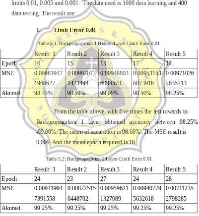
Analyzes of Backpropagation 1 hidden layer, 2 hidden layers and 3 hidden layers using 3 categories of weather output, there are clear, clouds and rain with a random weight of -1 to 1 and maximum epoch 5000 with error limits 0.01, 0.005 and 0.001. The data used is 1600 data learning and 400 data testing. The result are:
1. Limit Error 0.01
Table 5.1: Backpropagation 1 Hidden Layer-Limit Error 0.01
Result 1 Result 2 Result 3 Result 4 Result 5
Epoch 16 15 15 17 14
Akurasi 98.75% 98.50% 99.00% 98.50% 98.25%
From the table above, with five times the test towards to Backpropagation 1 layer obtained accuracy between 98.25% -99.00%. The mean of accuration is 98.60%. The MSE result is 0.009. And the mean epoch required is 16.
Table 5.2: Backpropagation 2 Layer-Limit Error 0.01
Result 1 Result 2 Result 3 Result 4 Result 5
Epoch 24 23 27 24 28
From the table above, with five experiments on Backpropagation 2 layer obtained the accuracy is 99.25% with mean MSE 0.008 and mean epoch 26.
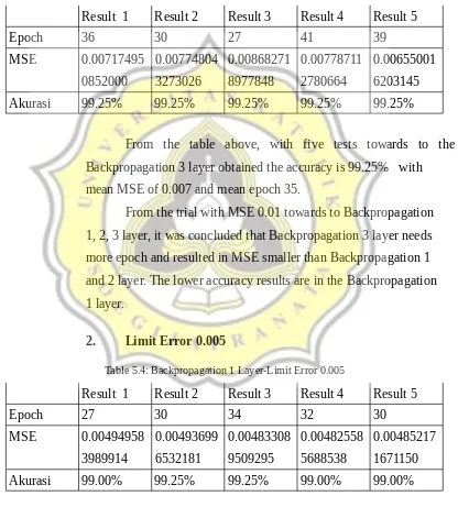
Table 5.3: Backpropagation 3 Layer-Limit Error 0.01
Result 1 Result 2 Result 3 Result 4 Result 5
Epoch 36 30 27 41 39
Akurasi 99.25% 99.25% 99.25% 99.25% 99.25%
From the table above, with five tests towards to the Backpropagation 3 layer obtained the accuracy is 99.25% with mean MSE of 0.007 and mean epoch 35.
From the trial with MSE 0.01 towards to Backpropagation 1, 2, 3 layer, it was concluded that Backpropagation 3 layer needs more epoch and resulted in MSE smaller than Backpropagation 1 and 2 layer. The lower accuracy results are in the Backpropagation 1 layer.
2. Limit Error 0.005
Table 5.4: Backpropagation 1 Layer-Limit Error 0.005
Result 1 Result 2 Result 3 Result 4 Result 5
Epoch 27 30 34 32 30
Akurasi 99.00% 99.25% 99.25% 99.00% 99.00%
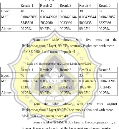
Table 5.5: Backpropagation 2 Layer-Limit Error 0.005
Result 1 Result 2 Result 3 Result 4 Result 5
Epoch 40 35 39 39 52
Akurasi 99.25% 99.25% 99.25% 99.25% 99.25%
From the table above, with five tests on the Backpropagation 2 layer, 99.25% accuracy is obtained with mean of MSE 0.0044 and mean of epoch 41.
Table 5.6: Backpropagation 3 Layer-Limit Error 0.005
Result 1 Result 2 Result 3 Result 4 Result 5
Epoch 46 48 66 35 49
Akurasi 99.25% 99.25% 99.25% 99.25% 99.25%
From the table above, with five tests against Backpropagation 3 layer 99.25% accuracy is obtained with mean MSE 0.0038 and mean epoch 49.
From a trial with MSE 0.005 limit to Backpropagation 1, 2, 3 layer, it was concluded that Backpropagation 3 layers require more epoch and produce smaller MSE than Backpropagation 1 and 2 layer. The lower accuracy results are in the Backpropagation 1 layer.
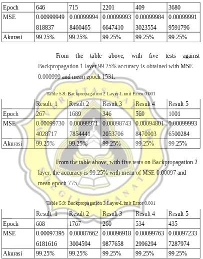
3. Limit Error 0.001
Table 5.7: Backpropagation 1 Layer-Limit Error 0.001
Epoch 646 715 2201 409 3680
Akurasi 99.25% 99.25% 99.25% 99.25% 99.25%
From the table above, with five tests against Backpropagation 1 layer 99.25% accuracy is obtained with MSE 0.000999 and mean epoch 1531.
Table 5.8: Backpropagation 2 Layer-Limit Error 0.001
Result 1 Result 2 Result 3 Result 4 Result 5
Epoch 267 1689 346 569 1001
MSE 0.00099730
Akurasi 99.25% 99.25% 99.25% 99.25% 99.25%
From the table above, with five tests on Backpropagation 2 layer, the accuracy is 99.25% with mean of MSE 0.00097 and mean epoch 775.
Table 5.9: Backpropagation 3 Layer-Limit Error 0.001
Result 1 Result 2 Result 3 Result 4 Result 5
Epoch 608 1767 260 534 435
MSE 0.00097395
Akurasi 99.25% 99.25% 99.25% 99.25% 99.25%
From the trial with the limit of MSE 0.001 to Backpropagation 1, 2 and 3 layer obtained the conclusion that Backpropagation with 3 layer produce MSE smaller than 1 and 2 layer. The accuracy results obtained on Backpropagation with 1, 2, 3 layer is the same that is 99.25%.
5.2.2 Backpropagation using Limitation Epoch
Analyzes of Backpropagation 1 hidden layer, 2 hidden layers and 3 hidden layers using 3 categories of weather output, there are clear, clouds and rain with a random weight of -1 to 1 and maximum epoch 50, 40 and 30. The data used is 1600 data learning and 400 data testing. The result are:
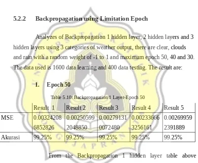
1. Epoch 50
Table 5.10: Backpropagation 1 Layer-Epoch 50
Result 1 Result 2 Result 3 Result 4 Result 5
MSE 0.00324208
Akurasi 99.25% 99.25% 99.25% 99.25% 99.25%
From the Backpropagation 1 hidden layer table above obtained the accuracy of 99.25%, the mean of MSE value is 0.002.
Table 5.11: Backpropagation 2 Layer-Epoch 50
Result 1 Result 2 Result 3 Result 4 Result 5
MSE 0.00317046
From the Backpropagation 2 hidden layer table above obtained an average accuracy of 99.15%, the mean of MSE value is 0.005.
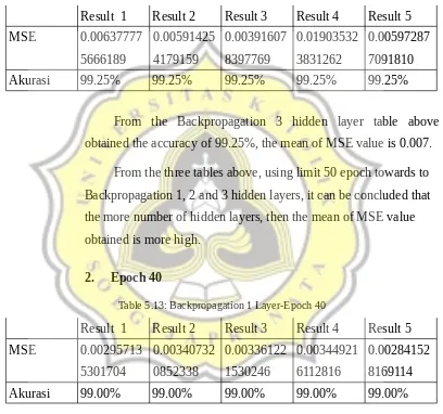
Table 5.12: Backpropagation 3 Layer-Epoch 50
Result 1 Result 2 Result 3 Result 4 Result 5
MSE 0.00637777
Akurasi 99.25% 99.25% 99.25% 99.25% 99.25%
From the Backpropagation 3 hidden layer table above obtained the accuracy of 99.25%, the mean of MSE value is 0.007.
From the three tables above, using limit 50 epoch towards to Backpropagation 1, 2 and 3 hidden layers, it can be concluded that the more number of hidden layers, then the mean of MSE value obtained is more high.
2. Epoch 40
Table 5.13: Backpropagation 1 Layer-Epoch 40
Result 1 Result 2 Result 3 Result 4 Result 5
MSE 0.00295713
Akurasi 99.00% 99.00% 99.00% 99.00% 99.00%
From the Backpropagation 1 hidden layer table above, the accuracy of 99.00% is obtained, the mean of MSE is 0.003.
Table 5.14: Backpropagation 2 Layer-Epoch 40
Result 1 Result 2 Result 3 Result 4 Result 5
Akurasi 99.00% 99.25% 99.25% 97.25% 99.25%
From the Backpropagation 2 hidden layer table above obtained the accuracy of 97.25%-99.25% that mean is 98.80%, the mean of MSE is 0.006.
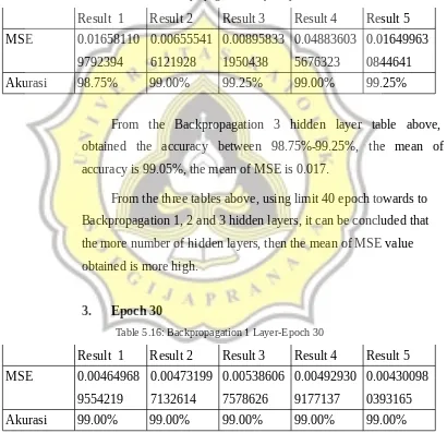
Table 5.15: Backpropagation 3 Layer-Epoch 40
Result 1 Result 2 Result 3 Result 4 Result 5
MSE 0.01658110
Akurasi 98.75% 99.00% 99.25% 99.00% 99.25%
From the Backpropagation 3 hidden layer table above, obtained the accuracy between 98.75%-99.25%, the mean of accuracy is 99.05%, the mean of MSE is 0.017.
From the three tables above, using limit 40 epoch towards to Backpropagation 1, 2 and 3 hidden layers, it can be concluded that the more number of hidden layers, then the mean of MSE value obtained is more high.
3. Epoch 30
Table 5.16: Backpropagation 1 Layer-Epoch 30
Result 1 Result 2 Result 3 Result 4 Result 5
MSE 0.00464968
Akurasi 99.00% 99.00% 99.00% 99.00% 99.00%
Table 5.17: Backpropagation 2 Layer-Epoch 30
Result 1 Result 2 Result 3 Result 4 Result 5
MSE 0.00790904
0683588
0.00510912 3532870
0.00839753 9510470
0.00360291 6404369
0.00898582 2373601
Akurasi 99.25% 99.25% 99.25% 99.25% 97.50%
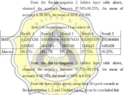
From the Backpropagation 2 hidden layer table above, obtained the accuracy between 97.50%-99.25%, the mean of accuracy is 98.90%, the mean of MSE is 0.006.
Table 5.18: Backpropagation 3 Layer-Epoch 30
Result 1 Result 2 Result 3 Result 4 Result 5
MSE 0.02613288
6393605
0.01459799 0647491
0.03079434 2890749
0.02603319 3249123
0.01464684 0481439
Akurasi 99.25% 99.25% 99.25% 97.75% 99.25%
From the Backpropagation 3 hidden layer table above, obtained the accuracy between 97.75%-99.25%, the mean of accuracy is 98.95%, the mean of MSE is 0.018.