A Journey from Robot to Digital Human

(1)

Modeling and Optimization in Science and Technologies

A Journey from

Robot to

Digital Human

Edward Y.L. Gu

Mathematical Principles and

Applications with MATLAB Programming

(2)

Modeling and Optimization in Science

and Technologies

Volume 1

Series Editors

Srikanta Patnaik (Editor-in-Chief) SOA University, Orissa, India

Ishwar K. Sethi

Oakland University, Rochester, USA

Xiaolong Li

Indiana State University, Terre Haute, USA

Editorial Board Li Cheng,

Department of Mechanical Engineering, The Hong Kong Polytechnic University, Hong Kong

Jeng-Haur Horng,

Department of Power Mechnical Engineering,

National Formosa University, Yulin,

Taiwan Pedro U. Lima,

Institute for Systems and Robotics, Lisbon,

Portugal

Mun-Kew Leong,

Institute of Systems Science, National University of Singapore Muhammad Nur,

Faculty of Sciences and Mathematics, Diponegoro Unersity,

Semarang, Indonesia

Kay Chen Tan,

Department of Electrical and Computer Engineering, National University of Singapore, Singapore

Yeon-Mo Yang,

Department of Electronic Engineering, Kumoh National Institute of Technology, Gumi, South Korea

Liangchi Zhang,

School of Mechanical and Manufacturing Engineering,

The University of New South Wales, Australia

Baojiang Zhong,

School of Computer Science and Technology, Soochow University, Suzhou, China

Ahmed Zobaa,

School of Engineering and Design, Brunel University, Uxbridge, Middlesex, UK

For further volumes:

(3)

About This Series

The book seriesModeling and Optimization in Science and Technologies (MOST)

(4)

Edward Y.L. Gu

A Journey from Robot to

Digital Human

Mathematical Principles and Applications with

MATLAB Programming

(5)

Edward Y.L. Gu

Dept. of Electrical and Computer Engineering

Oakland University Rochester, Michigan USA

ISSN 2196-7326 ISSN 2196-7334 (electronic) ISBN 978-3-642-39046-3 ISBN 978-3-642-39047-0 (eBook) DOI 10.1007/978-3-642-39047-0

Springer Heidelberg New York Dordrecht London Library of Congress Control Number: 2013942012

c

Springer-Verlag Berlin Heidelberg 2013

This work is subject to copyright. All rights are reserved by the Publisher, whether the whole or part of the material is concerned, specifically the rights of translation, reprinting, reuse of illustrations, recitation, broadcasting, reproduction on microfilms or in any other physical way, and transmission or information storage and retrieval, electronic adaptation, computer software, or by similar or dissimilar methodology now known or hereafter developed. Exempted from this legal reservation are brief excerpts in connection with reviews or scholarly analysis or material supplied specifically for the purpose of being entered and executed on a computer system, for exclusive use by the purchaser of the work. Duplication of this publication or parts thereof is permitted only under the provisions of the Copyright Law of the Publisher’s location, in its current version, and permission for use must always be obtained from Springer. Permissions for use may be obtained through RightsLink at the Copyright Clearance Center. Violations are liable to prosecution under the respective Copyright Law.

The use of general descriptive names, registered names, trademarks, service marks, etc. in this publication does not imply, even in the absence of a specific statement, that such names are exempt from the relevant protective laws and regulations and therefore free for general use.

While the advice and information in this book are believed to be true and accurate at the date of pub-lication, neither the authors nor the editors nor the publisher can accept any legal responsibility for any errors or omissions that may be made. The publisher makes no warranty, express or implied, with respect to the material contained herein.

Printed on acid-free paper

(6)

(7)

Preface

This book is intended to be a robotics textbook with an extension to digital human modeling and MATLABT M _{programming for both senior}

undergrad-uate and gradundergrad-uate engineering students. It can also be a research book for researchers, scientists, and engineers to learn and review the fundamentals of robotic systems as well as the basic methods of digital human modeling and motion generation. In the past decade, I wrote and annually updated two lecture notes: Robotic Kinematics, Dynamics and Control, and Modern Theories of Nonlinear Systems and Control. Those lecture notes were success-fully adopted by myself as the oﬃcial textbooks for my dual-level robotics course and graduate-level nonlinear control systems course in the School of Engineering and Computer Science, Oakland University. Now, the major sub-jects of those two lecture notes are systematically mixed together and further extended by adding more topics, theories and applications, as well as more examples and MATLABT M _{programs to form the first part of the book.}

I had also been invited and worked for the Advance Manufacturing Engi-neering (AME) of Chrysler Corporation as a summer professor intern for the past 12 consecutive summers during the 2000’s. The opportunity of working with the automotive industry brought to me tremendous real-world knowl-edge and experience that was almost impossible to acquire from the class-room. In more than ten years of the internship program and consulting work, I was personally involved in their virtual assembly and product design inno-vation and development, and soon became an expert in major simulation soft-ware tools, from IGRIP robotic models, the early product of Deneb Robotics (now Dassault/Delmia) to the Safework mannequins in CATIA. Because of this unique opportunity, I have already been on my real journey from robot to digital human.

(8)

VIII Preface

areas together, even though the latter often borrows the modeling theories and motion generation algorithms from the former.

Almost every chapter in the book has a section of exercise problems and/or computer projects, which will be beneficial for students to reinforce their understanding of every concept and algorithm. It is the instructor’s discretion to select sections and chapters to be covered in a single-semester robotics course. In addition, I highly recommend that the instructor teach students to write a program and draw a robot or a mannequin in MATLABT M _with

realistic motion by following the basic approaches and illustrations from the book.

I hereby acknowledge my indebtedness to the people who helped me with diﬀerent aspects of collecting knowledge, experience, data and programming skills towards the book completion. First, I wish to express my grateful appre-ciations to Dr. Leo Oriet who was the former senior manager when I worked for the AME of Chrysler Corporation, and Yu Teng who was/is a manager and leader of the virtual assembly and product design group in the AME of Chrysler. They both not only provided me with a unique opportunity to work on the digital robotic systems and human modeling for their ergonomics and product design verification and validation in the past, but also gave me ev-ery support and encouragement in recent years. I also wish to thank Michael Hicks who is an engineer working for General Dynamics Land Systems, and Ashley Liening who is a graduate student majoring in English at Oakland University for helping me polish my writing.

Furthermore, the author is under obligation to Fanuc Robotics, Inc., Robotics Research Corporation, and Aldebaran Robotics, Paris, France for their courtesies and permissions to include their photographs into the book.

Edward Y.L. Gu,Rochester, Michigan guy@oakland.edu

(9)

List of Figures

1.1 Married with a child . . . 2

1.2 A Fanuc M-900iB/700 industrial robot in drilling operation. Photo courtesy of Fanuc Robotics, Inc. . . 4

1.3 Robotics research and evolutions . . . 5

1.4 Important definitions in robotics . . . 8

2.1 Two parallel vectors have a common length . . . 16

2.2 Problem 2 . . . 44

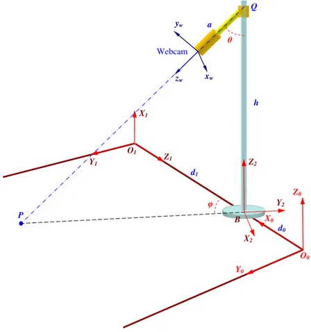
3.1 The webcam position and orientation . . . 52

3.2 Problem 1 . . . 77

3.3 Problem 3 . . . 78

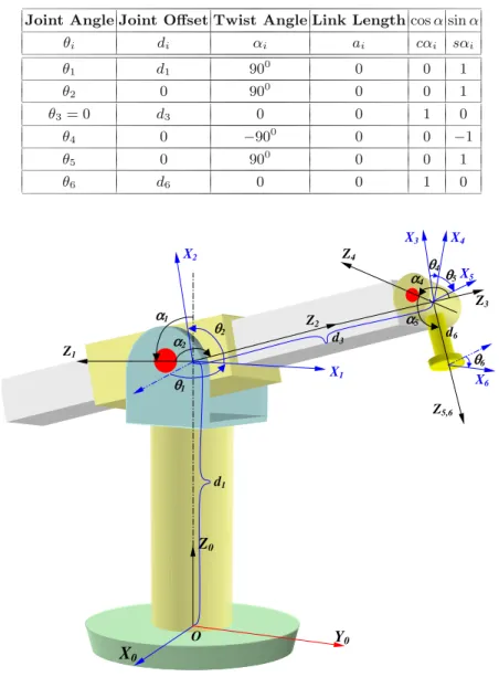
4.1 Definition of the Denavit-Hartenberg (D-H) Convention . . . 84

4.2 A 6-joint Stanford-type robot arm . . . 85

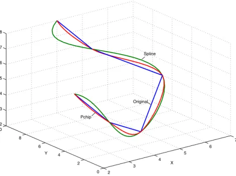
4.3 A curved path before and after the spline and pchip interpolations . . . 89

4.4 Example of the position and orientation path planning . . . . 90

4.5 Multi-configuration for a two-link arm . . . 94

4.6 Two robot arms with theirz-axes . . . 96

4.7 The first and second I-K solutions for the Stanford arm . . . 99

4.8 The third and fourth I-K solutions for the Stanford arm . . . 99

4.9 The motion of linknsuperimposed by the motion of linki . . . 103

4.10 An industrial robot model with coordinate frames assignment . . . 113

4.11 The Stanford-type robot is driving a screw into a workpiece . . . 116

4.12 A 3-joint RRR robot hanging a simple pendulum . . . 117

(14)

XIV List of Figures

4.14 A block diagram of robotic hybrid position/force

control . . . 125

4.15 A Stanford robot is sitting at the Home position and ready to move and draw on a board . . . 126

4.16 The Stanford robot is drawing a sine wave on the board . . . 127

4.17 The industrial robot model at the Starting and Ending positions . . . 128

4.18 Robot 1 . . . 129

4.19 Robot 2 . . . 130

4.20 Robot 3 . . . 130

4.21 A 2-joint prismatic-revolute planar arm . . . 132

4.22 A 3-joint RPR robot arm . . . 133

4.23 A beam-sliding 3-joint robot . . . 134

5.1 Geometrical decomposition of the general solution . . . 138

5.2 A 7-joint redundant robot arm . . . 143

5.6 A three-joint RRR planar redundant robot arm . . . 146

5.7 Simulation results - only the rank (minimum-Norm) solution . . . 147

5.8 Simulation results - both the rank and null solutions . . . 148

5.9 The 7-joint robot arm is hitting a post when drawing a circle . . . 149

5.10 The 7-joint robot is avoiding a collision by a potential function optimization . . . 149

5.11 A top view of the 7-joint redundant robot with a post and a virtual point . . . 151

5.12 The Stanford-type robot arm is sitting on a wheel mobile cart . . . 155

5.13 A hybrid-chain planar robot . . . 157

5.14 Stewart platform - a typical 6-axis parallel-chain system . . . 157

5.15 A 7-axis dexterous manipulator RRC K-1207 and a dual-arm 17-axis dexterous manipulator RRC K-2017. Photo courtesy of Robotics Research Corporation, Cincinnati, OH. . . 158

5.16 Kinematic model of the two-arm 17-joint hybrid-chain robot . . . 159

5.17 A two-robot coordinated system . . . 163

5.18 A Nao-H25 humanoid robotic system. Photo courtesy of Aldebaran Robotics, Paris, France. . . 164

5.19 A 6-axis 6-6 parallel-chain hexapod system . . . 165

(15)

List of Figures XV

5.21 Solution to the forward kinematics of the Stewart

platform . . . 169

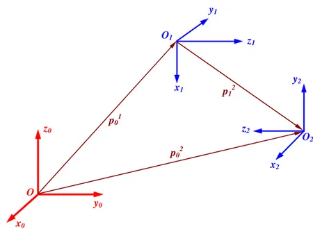
5.22 The definitions ofpi 6’s on the top mobile disc. They are also applicable topi 0’s on the base disc of the 6-6 Stewart platform. . . 178

5.23 Two types of the 3-parallel mechanism . . . 184

5.24 Kinematic analysis of a 3-leg UPS platform . . . 186

5.25 Top revolute-joint configurations . . . 187

5.26 Solve the I-K problem for a 3+3 hybrid robot . . . 191

5.27 Delta URR vs. UPR 3-leg parallel system . . . 194

5.28 A three-joint RPR planar robot arm . . . 197

5.29 A 3+3 hybrid robot in rectangle configuration . . . 198

5.30 A 4-joint beam-hanging PRRP robot . . . 199

5.31 An RRP 3-joint planar robot to touch a bowl . . . 199

5.32 An RPR 3-joint planar robot . . . 200

5.33 A planar mechanism . . . 200

5.34 Three parallel-chain systems . . . 201

6.1 Data structure of a cylinder drawing in MATLABT M _{. . . . .} ₂₀₆

6.2 Data structure of a sphere drawing in MATLABT M_{. . . .} ₂₀₈

6.3 A diamond and an ellipsoid drawing in MATLABT M _{. . . . .} ₂₀₉

6.4 Create a rectangular surface in MATLABT M _{. . . .} ₂₁₀

6.5 Create a full torus surface in MATLABT M _{. . . .} ₂₁₁

6.6 Create a half torus surface in MATLABT M _{. . . .} ₂₁₂

6.7 Making a local deformation for a cylindrical surface in MATLABT M _{. . . .} ₂₁₃

6.8 Sending an object from the base to a desired destination . . . 214

6.9 D-H modeling of the 7-joint redundant robot . . . 215

6.10 A Stewart platform and coordinate frames assignment . . . . 218

6.11 The Stewart platform in motion . . . 222

6.12 A two-arm robot at its Home position . . . 223

6.13 A two-arm robot is picking up a disc from the floor . . . 223

6.14 A two-arm robot is hanging the disc on the wall . . . 224

6.15 A 3+3 hybrid robot with equilateral triangle configuration at its Home position . . . 225

6.16 The 3+3 hybrid robot with equilateral triangle configuration starts drawing a sine wave . . . 226

6.17 The 3+3 hybrid robot with equilateral triangle configuration ends the drawing . . . 227

6.18 A 3+3 hybrid robot with rectangle configuration at its Home position . . . 227

(16)

XVI List of Figures

7.1 Two 6-revolute-joint industrial robots: Fanuc R-2000iB (left) and Fanuc M-900iA (right). Photo courtesy of Fanuc

Robotics, Inc. . . 234

7.2 RR-type and RP-type 2-link robots . . . 234

7.3 C-manifolds for RR-type and RP-type 2-link robots . . . 235

7.4 A rigid body and its reference frame changes . . . 239

7.5 Getting-busier directions for kinematics and dynamics . . . . 240

7.6 Force/torque analysis of linki. . . 241

7.7 Velocity analysis of a three-joint planar robot arm . . . 247

7.8 An inertial matrix W is formed by stacking every Wj together . . . 251

7.9 Axes assignment of the three-joint planar robot . . . 251

7.10 The cylindrical and spherical local coordinate systems . . . 259

7.11 Diﬀerent mapping cases fromS1 _{to Euclidean spaces . . . .} ₂₆₃

7.12 A 2D torusT2 situated in Euclidean spacesR3 _andR2_{. . . .} ₂₆₃

7.13 A planar RR-type arm and its C-manifold as a flatted torus . . . 264

7.14 The first and second of four I-K solutions for a Stanford arm . . . 274

7.15 The third and forth of four I-K solutions for a Stanford arm . . . 274

7.16 An inverted pendulum system . . . 278

7.17 The minimum embeddable C-manifold of the inverted pendulum system . . . 278

7.18 An RRR-type planar robot and its multi-configuration . . . . 280

8.1 A joint path example without and with cubic spline function . . . 295

8.2 Joint position and velocity profiles for the second spline function . . . 296

8.3 A DC-motor electrical and mechanical model . . . 298

8.4 A block diagram of the DC-motor model . . . 300

8.5 A block diagram of DC-motor position-feedback control . . . 301

8.6 A block diagram for an input-state linearized system . . . 316

8.7 A block diagram for an input-output linearized trajectory-tracking system . . . 323

8.8 A block diagram for a partially input-output linearized system . . . 329

8.9 The block diagram of a single feedback loop . . . 333

8.10 Model a ball-board control system using the robotic D-H convention . . . 334

8.11 The ball is at an initial position to start tracking a sine wave on the board . . . 341

(17)

List of Figures XVII

8.13 The ball is now on the track by controlling the board

orientation . . . 341

8.14 The ball is well controlled to continue tracking the sine wave on the board . . . 342

8.15 The ball is successfully reaching the end of the sine wave on the board . . . 342

8.16 An energy-like functionV(x) and a V-lifted trajectory . . . . 348

8.17 A flowchart of the backstepping control design approach . . . 365

8.18 A flowchart of backstepping control design for ak-cascaded dynamic system . . . 369

8.19 A block diagram of adaptive control design . . . 372

8.20 An RRP type three-joint robot arm . . . 378

8.21 The simulation results with M3 as the minimum embeddable C-manifold . . . 385

8.22 A 3-joint Stanford-like robot arm . . . 386

8.23 A 2-joint robot arm sitting on a rolling log . . . 388

8.24 A 3-piston parallel-chain planar robot . . . 389

8.25 A block diagram of the DC-motor in driving a robotic link . . . 391

9.1 Major joints and types over an entire human body . . . 398

9.2 The real human vertebral column and its modeling . . . 399

9.3 A block diagram of digital human joint distribution . . . 400

9.4 Coordinate frame assignment on a digital mannequin . . . 402

9.5 The left arm of a digital mannequin is manually maneuvered by a local I-K algorithm with at least two distinct configurations . . . 412

9.6 A block diagram of the five-point model . . . 421

9.7 Shoulder abduction and its clavicle joint combination eﬀect . . . 424

9.8 Hip flexion and abduction with joint combination eﬀects to the trunk flexion and lateral flexion . . . 425

9.9 Two-joint muscles on the arm and leg . . . 425

9.10 The angles of human posture in sagittal plane for a joint strength prediction . . . 433

9.11 A closed boundary for the shoulder ROM and ROS in a chart of joint torque vs. joint angle . . . 435

9.12 Analysis of mannequin force balance in standing posture . . . 437

9.13 Two arms and torso joint torque distribution in standing posture . . . 438

9.14 A complete joint torque distribution in standing posture . . . 440

9.15 Analysis of mannequin force balance in sitting posture . . . . 441

(18)

XVIII List of Figures

9.17 The joint torque distribution over two arms and torso in

sitting posture . . . 442

9.18 A complete joint torque distribution in sitting posture . . . . 443

9.19 The joint torque distribution over two arms and torso in kneeling posture . . . 444

9.20 A complete joint torque distribution in kneeling posture . . . 445

9.21 A digital human skeleton model with segment numbering . . . 447

9.22 A mannequin is in neutral standing posture and ready to pick an object . . . 450

9.23 A 47-joint torque distribution due to gravity in neutral standing posture . . . 450

9.24 A 47-joint torque distribution due to gravity in standing posture before the balance . . . 451

9.25 A 47-joint torque distribution due to gravity after balancing the reaction forces . . . 451

9.26 Mannequin postures in picking up a load without and with optimization . . . 459

9.27 A joint torque distribution due to weight-lift without and with optimization . . . 460

9.28 A complete joint torque distribution with and without optimization . . . 460

9.29 The mannequin postures in placing a load on the overhead shelf without and with optimization . . . 461

9.30 A joint torque distribution in placing a load with and without optimization . . . 461

9.31 A complete joint torque distribution with and without optimization . . . 462

10.1 A digital human head model . . . 468

10.2 A face picture for texture-mapping onto the surface of a digital human head model . . . 469

10.3 A digital human abdomen/hip model . . . 475

10.4 A digital human torso model . . . 476

10.5 A digital human upper arm/forearm model . . . 476

10.6 A digital human thigh/leg model . . . 477

10.7 Three diﬀerent views of the finally assembled digital human model . . . 480

10.8 A skeletal digital mannequin in dancing . . . 483

10.9 A block diagram for the right hand modeling and reversing the order for the left hand . . . 483

(19)

List of Figures XIX

10.11 The right hand digital model with a ball-grasping

gesture . . . 488

10.12 The left hand digital model with a ball-grasping gesture . . . 488

10.13 A digital hand model consists of various drawing components . . . 490

10.14 The right hand is going to grasp a big ball . . . 493

10.15 A walking z-coordinates profile for the hands and feet from a motion capture . . . 498

10.16 A walkingx-coordinates profile for the feet from a motion capture . . . 499

10.17 A walkingx-coordinates profile for the hands from a motion capture . . . 499

10.18 A walkingx-coordinates profile for the feet created by a numerical algorithm . . . 501

10.19 A walkingx-coordinates profile for the hands created by a numerical algorithm . . . 502

10.20 A walkingz-coordinates profile for both the feet and hands created by a numerical algorithm . . . 502

10.21 z-trajectories in a running case for the feet and hands created by a numerical model . . . 503

10.22 A digital human in walking . . . 504

10.23 A digital human in running . . . 504

10.24 z-trajectories in a jumping case for the feet and hands by a motion capture . . . 505

10.25 x-trajectories in a jumping case for the two feet by a motion capture . . . 505

10.26 x-trajectories in a jumping case for the two hands by a motion capture . . . 506

10.27 xandz-trajectories in a jumping case for the H-triangle by a motion capture . . . 506

10.28 A digital human in jumping . . . 507

10.29 A relation diagram between the human centered frame and the world base . . . 511

10.30 A digital human in running and ball-throwing . . . 513

10.31 A digital human in ball-throwing . . . 513

10.32 A digital human in ball-throwing . . . 514

10.33 A digital human is climbing up a stair . . . 514

10.34 A digital human is climbing up a stair and then jumping down . . . 515

10.35 A digital human is jumping down from the stair . . . 515

10.36 A digital human in springboard diving . . . 516

(20)

XX List of Figures

10.41 A digital human is getting into the car . . . 518 10.42 A digital human is getting and seating into the car . . . 518 10.43 z-trajectories in the ball-throwing case for the feet and

hands by the motion capture . . . 519 10.44 x-trajectories in the ball-throwing case for the two feet by

the motion capture . . . 519 10.45 x-trajectories in the ball-throwing case for the two hands

by the motion capture . . . 520 10.46 xand z-trajectories in the ball-throwing case for the

H-triangle by the motion capture . . . 520 10.47 z-trajectories in the stair-climbing/jumping case for the

feet and hands by the motion capture . . . 521 10.48 x-trajectories in the stair-climbing/jumping case for the

two feet by the motion capture . . . 522 10.49 x-trajectories in the stair-climbing/jumping case for the

two hands by the motion capture . . . 523 10.50 xandz-trajectories in the stair-climbing/jumping case for

the H-triangle by the motion capture . . . 523 10.51 x-trajectories in the springboard diving case for the two

feet by a math model . . . 524 10.52 x-trajectories in the springboard diving case for the two

hands by a math model . . . 525 10.53 z-trajectories in the springboard diving case for the two

feet and two hands by a math model . . . 525 10.54 x-trajectories in the ingress case for the two feet by a

math model . . . 527 10.55 x-trajectories in the ingress case for the two hands by a

math model . . . 528 10.56 y-trajectories in the ingress case for the two feet by a

math model . . . 528 10.57 y-trajectories in the ingress case for the two hands by a

math model . . . 529 10.58 z-trajectories in the ingress case for the two feet and two

hands by a math model . . . 529

11.1 A structure of digital human dynamic model and motion

drive . . . 535 11.2 Dynamic balance in standing case andδ-force excitation

in a walking case . . . 541 11.3 Dynamic balance andδ-force excitation in

a running case . . . 542 11.4 A frontal collision acceleration profile as a vehicle speed at

45 mph . . . 544 11.5 The mannequin forgets wearing an upper seat belt before

(21)

List of Figures XXI

11.6 At the moment of collision, the mannequin’s chest Hits

the steering wheel . . . 547 11.7 After the chest impact, the head immediately follows to

hit the steering wheel . . . 547 11.8 The mannequin’s head is bouncing back after hitting the

steering wheel . . . 548 11.9 With the momentum of bouncing back, the mannequin’s

head and back hit the car seat back . . . 548 11.10 The mannequin now wears both upper and lower seat

belts and drives the car at 45 mph . . . 549 11.11 After a frontal impact occurs, the mannequin’s chest hits

the activated frontal airbag . . . 549 11.12 With the airbag, the mannequin’s chest and head are

protected from the deadly hit . . . 550 11.13 Under an active restraint control, the mannequin is much

safer in a crash accident . . . 550 11.14 With the active restraint control, severe bouncing back to

hit the car seat back is also avoided . . . 551 11.15 The lumbar, thorax and head accelerations in Case 1 . . . 552 11.16 The lumbar, thorax and head accelerations in Case 2 . . . 552 11.17 The lumbar, thorax and head accelerations in the case

with active restraint control . . . 553 11.18 The control inputs in the case with an active restraint

system . . . 553 11.19 The acceleration profile of an IED explosion underneath

the vehicle seat . . . 554 11.20 A digital warfighter is sitting in a military vehicle with a

normal posture . . . 556 11.21 An IED explosion blasts the vehicle and bounces up the

mannequin . . . 557 11.22 The explosion makes the mannequin further jump up . . . 557 11.23 The head would severely hit the steering wheel without

any protection in response to the IED explosion . . . 558 11.24 The digital warfighter is sitting with a 200_{turning angle}

before an IED explodes . . . 558 11.25 The digital warfighter body is not only bouncing up, but

also starting leaning oﬀ . . . 559 11.26 The digital warfighter is further leaning away . . . 559 11.27 The digital warfighter is struggling and finally falling

down from the seat . . . 560 11.28 Three joint accelerations of the neck vs. time under an

(22)

XXII List of Figures

11.29 Three joint accelerations of the neck vs. time under an

initial posture with a 200 _{turning angle . . . .} ₅₆₁ 11.30 A typical seat-belt restraint system . . . 563 11.31 A complete block diagram for the active restraint control

system . . . 568 11.32 A digital human drives a car with an active suspension

system . . . 572 11.33 A future integration in research and development of digital

(23)

Chapter 1 Introduction to Robotics and Digital

Human Modeling

1.1 Robotics Evolution: The Past, Today and

Tomorrow

Robotics research and technology development have been on the road to grow and advance for almost half a century. The history of expedition can be divided into three major periods: the early era, the middle age and the recent years. The oﬃcial definition of robot by the Robot Institute of America (RIA) early on was:

“A robot is a reprogrammable multi-functional manipulator de-signed to move material, parts, tools, or specialized devices through variable programmed motions for the performance of a variety of tasks.”

Today, as commonly recognized, beyond such a professional definition from history, the general perception of a robot is a manipulatable system to mimic a human with not only the physical structure, but also the intelligence and even personality. In the early era, people often remotely manipulated material via a so-called teleoperator as well as to do many simple tasks in industrial applications. The teleoperator was soon “married” with the computer numer-ically controlled (CNC) milling machine to “deliver” a new-born baby that was the robot, as depicted in Figure 1.1.

Since then, the robots were getting more and more popular in both indus-try and research laboratories. A chronological overview of the major historical events in robotics evolution during the early era is given as follows:

1947- The 1st servoed electric powered teleoperator was developed; 1948- A teleoperator was developed to incorporate force feedback; 1949- Research on numerically controlled milling machines was initiated; 1954- George Devol designed the first programmable robot;

1956- J. Engelberger bought the rights to found Unimation Co. and produce the Unimate robots;

1961- The 1st Unimate robot was installed in a GM plant for die casting; 1961- The 1st robot incorporating force feedback was developed;

1963- The 1st robot vision system was developed;

E.Y.L. Gu,A Journey from Robot to Digital Human, 1

Modeling and Optimization in Science and Technologies 1,

(24)

2 1 Introduction to Robotics and Digital Human Modeling

Teleoperators

(TOP)

Numerical

Controlled Milling

Machines

M

Robot

Fig. 1.1 Married with a child

1971- The Stanford arm was developed at Stanford University;

1973- The 1st robot programming language (WAVE) was developed at Stanford University;

1974- Cincinnati Milacron introduced the T3 robot with Computer Con-trol;

1975- Unimation Inc. registered its first financial profit;

1976- The RCC (Remote Center Compliance) device for part insertion was developed at Draper Labs;

1978- Unimation introduced the PUMA robot based on a GM study; 1979- The SCARA robot design was introduced in Japan;

1981- The 1st direct-drive robot was developed at Carnegie-Mellon Univer-sity.

Those historical and revolutionary initiations are unforgettable, and almost every robotics textbook acknowledges and refers to the glorious childhood of industrial robots [1, 2, 3]. Following the early era of robotics, from 1982 to 1996 at the middle age of robotics, a variety of new robotic systems and their kinematics, dynamics, and control algorithms were invented and extensively developed, and the pace of growth was almost exponential. The most signif-icant findings and achievements in robotics research can be outlined in the following representative aspects:

• The Newton-Euler inverse-dynamics algorithm;

• Extensive studies on redundant robots and applications;

• Study on multi-robot coordinated systems and global control of robotic groups;

• Control of robots with flexible links and/or flexible joints;

• Research on under-actuated and floating base robotic systems;

• Study on parallel-chain robots versus serial-chain robots;

(25)

1.1 Robotics Evolution: The Past, Today and Tomorrow 3

• Development of advanced force control algorithms and sensory devices;

• Sensory-based control and sensor fusion in robotic systems;

• Robotic real-time vision and pattern recognition;

• Development of walking, hopping, mobile, and climbing robots;

• Study on hyper-redundant (snake-type) robots and applications;

• Multi-arm manipulators, reconfigurable robots and robotic hands with dexterous fingers;

• Wired and Wireless networking communications for remote control of robotic groups;

• Mobile robots and field robots with sensor networks;

• Digital realistic simulations and animations of robotic systems;

• The study of bio-mimic robots and micro-/nano-robots;

• Research and development of humanoid robots;

• Development and intelligent control of android robots, etc.

After 1996, robotics research has advanced into its maturity. The robotic applications were making even larger strides than the early era to continu-ously grow and rapidly deploy the robotic technologies from industry to many diﬀerent fields, such as the military applications, space exploration, under-ground and underwater operations, medical surgeries as well as the personal services and homeland security applications. In order to meet such a large va-riety of challenges from the applications, robotic systems design and control have been further advanced to a new horizon in the recent decades in terms of their structural flexibility, dexterity, maneuverability, reconfigurability, scal-ability, manipulscal-ability, control accuracy, environmental adaptability as well as the degree of intelligence [4]–[8]. One can witness the rapid progress and great momentum of this non-stop development in the large volume of inter-net website reports. Figure 1.2 shows a new Fanuc M-900iB/700 super heavy industrial robot that oﬀers 700 Kg. payload capacity with built-in iRVision and force sensing integrated systems.

Parallel to the robotics research and technology development, virtual robotic simulation also has a long history of expedition. In the mid-1980’s, Deneb Robotics, known as Dassault/Delmia today, released their early ver-sion of a robot graphic simulation software package, called IGRIP. Nearly as the same time, Technomatix (now UGS/Technomatix) introduced a ROBO-CAD product, which kicked oﬀ a competition. While both the major robotic simulation packages impressed the users with their 3D colorful visualizations and realistic motions, the internal simulation algorithms could not accurately predict the reaching positions and cycle times, mainly due to the parameter uncertainty. As a result of the joint eﬀort between the software firms and robotic manufacturers, a Realistic Robot Simulation (RRS) specification was created to improve the accuracy of prediction.

(26)

be-4 1 Introduction to Robotics and Digital Human Modeling

Fig. 1.2 A Fanuc M-900iB/700 industrial robot in drilling operation. Photo

cour-tesy of Fanuc Robotics, Inc.

came more capable of managing product design in association with the man-ufacturing processes from concept to prototyping, to production. Today, the status of robotic simulation has further advanced to a more sophisticated and comprehensive new stage. It has become a common language to com-municate design issues between the design teams and customers, and also an indispensable tool for product and process design engineers and managers as well as researchers to verify and validate their new concepts and findings.

The new trends of robotics research, robotic technology development and applications today and tomorrow will possibly grow even faster and be more flexible and dexterous in mechanism and more powerful in intelligence. Due to the potentially huge market and social demand, robotic systems design, performance, and technology have already jumped into a new transitional era from industrial and professional applications to social and personal ser-vices. Facing the pressing competitions and challenges from the transition, robotics research will never be running behind. Instead, by keeping up the great momentum of growth, it will rapidly move forward to create better solutions, make more innovations and achieve new findings to speed up the robotic technology development in the years to come [9]–[12].

(27)

1.1 Robotics Evolution: The Past, Today and Tomorrow 5

Intelligent

Service Robots

Industrial

Robots

Digital Human

Physical Models

& Motions

Humanoid

Robots

Mobile

Robots

Field

Robots

Non-Robotic

Systems

Control App.

Robotics

Research

Flexible

Automation

Walking

Robots

Smart Digital

Human

Integration

Home

Robots

Fig. 1.3 Robotics research and evolutions

growing and getting mature, it became more capable of helping new robotic systems creation and fueling new research branches to sprout and grow. In addition to creating and developing a variety of service robots, a number of new research and application branches have also been created and fed by the robotic systematic modeling approaches and control theories, which benefited their developments. One of those beneficiaries is digital human modeling and applications. The others may include many non-robotic systems dynamic modeling and control strategy design, such as a gun-turret control system for military vehicles, helicopters and platforms, and a ball-board control system that will be discussed in Chapter 8.

(28)

to weld and fabricate car bodies in an automotive body-in-white assembly station.

One of the most remarkable achievements that deserves celebration is the development of humanoid robots, which underlies an infrastructure of var-ious service robots and home robots. The history of the humanoid robot development is even longer than the industrial robots [15]. An Italian math-ematician/engineer Leonardo da Vinci designed a humanoid automaton that looks like an armored knight, known as Leonardo’s robot in 1495. The more contemporary human-like machine Wabot-1 was built at Waseda University in Tokyo, Japan in 1973. Wabot-1 was able to walk, to communicate with a person in Japanese by an artificial mouth, and to measure distances and directions to an object using external receptors, such as artificial ears and eyes. Ten years later, they created a new Wabot-2 as a musician humanoid robot that was able to communicate with a person, read a normal musical score by his eyes and play tones of average diﬃculty on an electronic organ. In 1986, Honda developed seven biped robots, called E0 (Experimental Model 0) through E6. Model E0 was created in 1986, E1-E3 were built between 1987 and 1991, and E4-E6 were done between 1991 and 1993. Then, Honda upgraded the biped robots to P1 (Prototype Model 1) through P3, as an evolutionary model series of the E series, by adding upper limbs. In 2000, Honda completed its 11th biped humanoid robot, known as ASIMO that was not only able to walk, but also to run.

Since then, many companies and research institutes followed to introduce their respective models of humanoid robots. A humanoid robot, called Ac-troid, which was covered by silicone “skin” to make it look like a real human, was developed by Osaka University in conjunction with Kokoro Company, Ltd. in 2003. Two years later, Osaka University and Kokoro developed a new series of ultra-realistic humanoid robots in Tokyo. The series initial model was Geminoid HI-1, followed by Geminoid-F in 2010 and Geminoid-DK in 2011.

It is also worth noting that in 2006, NASA and GM collaborated to de-velop a very advanced humanoid robot, called Robonaut 2. It was originally intended to assist astronauts in carrying out scientific experiments in a space shuttle or in the space station. Therefore, Robonaut 2 has only an upper body without legs for use in a gravity-free environment to perform advanced manipulations using its dexterous hands and arms [16, 17].

(29)

1.2 Digital Human Modeling: History, Achievements and New Challenges 7

in the home. However, to achieve this goal, only making a technological devel-opment eﬀort is not enough. Instead, it must also rely on more new findings and solutions in theoretical development and basic research to overcome every challenging hurdle.

As a summary, in the recent status of basic research in robotics, there is a number of topics that still remain open:

1. Adaptive control of under-actuated robots or robotic systems under non-holonomic constraints;

2. Dynamic control of flexible-joint and/or flexible-link robots;

3. The dual relationship between open serial and closed parallel-chain robots; 4. Real-time image processing and intelligent pattern recognition;

5. Stability of robotic learning and intelligent control;

6. Robotic interactions and adaptations to complex environments;

7. Perceptional performance in a closed feedback loop between robot and environment;

8. Cognitive interactions with robotic physical motions;

9. More open topics in robot dynamic control and human-machine interac-tions.

In conclusion, the robot analysis part of this book is intended to moti-vate and encourage the reader to accept all the new challenges and make every eﬀort and contribution to the current and future robotics research, sys-tems design and applications. The robotics part of the book will cover and focus primarily on the three major fundamental topics: kinematics, dynam-ics, and control, along with the related MATLABT M _programming.

Specif-ically, Figure 1.4 illustrates the formal definitions in the covered topics of robotics. However, the book does not intend to include discussions on robotic force control, learning and intelligent control, robotic vision and recogni-tion, sensory-feedback control, and programmable logic controller (PLC) and human-machine interface (HMI) based networking control of robotic groups. The reader can refer to the literature or application documents to learn more about those application-oriented topics.

1.2 Digital Human Modeling: History, Achievements

and New Challenges

(30)

Inverse Kinematics

Inverse Dynamics

Task Description

Cartesian Position

& Velocity

Joint Variables

Joint Torques

Cartesian

Forces

Task/Path Planning

Forward Kinematics

Forward Dynamics

Statics

General Definitions of Robotic Kinematics, Dynamics and Statics

Fig. 1.4 Important definitions in robotics

1. Experts in ergonomics can simulate and test various underlying human behavior theories with these models, thus better prioritizing areas of new research;

2. Experts can use the models to gain confidence about their own knowledge regarding people’s performance under a variety of circumstances;

3. The models provide a means to better communicate human performance attributes and capabilities to others who want to consider ergonomics in proposed designs.

Due to the limitation of computer power, the early attempt of digital human physical modeling was undertaken only conceptually until the late 1970’s. With the exponential growth of computational speed, memory and graphic performance, a mannequin and its motion could be realistically visu-alized in a digital environment to allow the ergonomics specialists, engineers, designers and managers to more eﬀectively assess, evaluate and verify their theoretical concepts, product designs, job analysis and human-involved pilot operations.

(31)

1.2 Digital Human Modeling: History, Achievements and New Challenges 9

Interaction Evaluation) was developed in the United Kingdom at that time and is now one of the leading packages in the world to run digital human simulations. During the late 1980’s, Safework and Jack were showing their new mannequins with real-time motions as well as their unique features and functions. In the early 1990’s, a human musculoskeletal model was developed in a digital environment by AnyBody Technology in Denmark to simulate a variety of work activities for automotive industry applications [18].

One of the most remarkable achievements in recent digital human modeling history was the research and development of a virtual soldier model: Santos in Center for Computer Aided Design at the University of Iowa, led by Dr. Karim Abdel-Malek during the 2000’s [22, 23, 24]. It is now under continu-ous development in a spin-oﬀ company SantosHuman, Inc. Not only has the Santos mannequin demonstrated its unique high-fidelity of appearance with deformable muscle and skin in a digital environment, but it has also made a pioneering leap and contribution to the digital human research community in borrowing and applying robotic modeling theories and approaches. Their multi-disciplinary research has integrated many major areas in digital human modeling and simulation, such as:

• Human performance and human systems integration;

• Posture and motion prediction;

• Task simulation and analysis;

• Muscle and physiological modeling;

• Dynamic strength and fatigue analysis;

• Whole body vibrations;

• Body armor design and analysis;

• Warfighter fightability and survivability;

• Clothing and fabric modeling;

• Hand modeling;

• Intuitive interfaces.

To model and simulate dynamics, one of the most representative software tools is MADYMO (Mathematical Dynamic Models) [20]. MADYMO was developed as a digital dummy for car crash simulation studies by the Nether-lands Organization for Applied Scientific Research (TNO) Automotive Safety Solutions division (TASS) in the early 1990’s. It oﬀers several digital dummy models that can be visualized in real-time dynamic responses to a collision. It also possesses a powerful post-processing capability to make a detailed analy-sis and check the results against the safety criteria and legal requirements. In addition, MADYMO provides a useful simulation tool of airbag and seat-belt design as well as the reconstruction and analysis of real accidents.

(32)

1. Although the realism of digital human appearance has made a break-through, the high-fidelity of digital human motion may need more improve-ments, especially in a sequential motion, high-speed motion and motion in complex restricted environments;

2. Further eﬀorts need to be made for modeling human-environment interac-tions in a more eﬀective and adaptive fashion;

3. More work must be done to enhance the digital human physical models in adapting to the complex anthropometry, physiology and biomechanics, as well as taking digital human vision and sound responses into modeling consideration;

4. Develop a true integration between the digital human physical and non-physical models in terms of psychology, feeling, cognition and emotion.

1.3 A Journey from Robot Analysis to Digital Human

Modeling

After screening the history and evolution of research and technology devel-opment in both robotics and digital human modeling, it is foreseeable that all progresses and cutting-edge innovations can always be mirrored in leading commercial simulation software products. However, most of such graphic sim-ulation packages render a small “window” as a feature of open architecture to allow the user to write his/her own application program for research, testing or verification. When the user’s program is ready to communicate the prod-uct, it often requires a special API (Application Program Interface) in order to acknowledge and run the user’s application program. Thus, it becomes very limited and may not be suitable for academic research and education. Therefore, it is ideal to place the modeling, programming, modification, re-finement and graphic animation all in one, such as MATLABT M_{, to create}

a flexible, user-friendly and true open-architectural digital environment for future robotics and digital human graphic simulation studies.

This book aims to take a journey from robot to digital human by providing the reader with a means to build a theoretical foundation at the beginning. Then, the reader will be able to mock up a desired 3D solid robot model or a mannequin in MATLABT M _{and drive it for motion. It will soon be}

real-ized that writing a MATLABT M _{code may not be diﬃcult, because it is the}

highest-level computer language. The most challenging issue is the necessary mathematical transformations behind the robot or mannequin drawing. This is the sole reason why the theoretical foundation must be built up before writ-ing a MATLABT M _{program to create a desired digital model for animation.}

Since MATLABT M _{has recently added a Robotics toolbox into the family,}

(33)

1.3 A Journey from Robot Analysis to Digital Human Modeling 11

Therefore, to make the journey more successful and exciting, this book will specifically focus on the basic digital modeling procedures, motion algorithms and optimization methodologies in addition to the theoretical fundamentals in robotic kinematics, statics, dynamics, and control. Making a realistic ap-pearance, adapting various anthropometric data and digital human cognitive modeling will not be the emphasis in this book. Instead, once a number of surfaces are created to be further assembled together, more time can always be spent to sculpture each surface more carefully and microscopically to make it look like a real muscle/skin as long as the surface has a suﬃcient enough resolution. Moreover, one can also concatenate the data between the adjacent surfaces to generate a certain eﬀect of deformation. For this reason, this book will introduce a few examples of basic mathematical sculpturing and deform-ing algorithms as a typical illustration, and leave to the reader to extend the basic algorithms to more advanced and sophisticated programs.

Furthermore, in the digital human modeling part of the book, each set of kinematic parameters, such as joint offsets and link lengths for a digital man-nequin is part of the anthropometric data. They can be easily set or reset from one to another in a modeling program, and the parameter exchange will never alter the kinematic structure. For example, when evaluating the joint torque distribution by statics for a digital human in operating a material-handling task, it is obvious that the result will be different from a different set of kine-matic parameters. However, once entering a desired set of parameters, the resulting joint torque distribution should exactly reflect the person’s perfor-mance under the particular anthropometric data. There is a large number of anthropometry databases available now [20], such as CAESAR, DINED, A-CADRE, U.S. Army Natick, NASA STD3000, MIL-STD-1472D, etc. The reader can refer to those documents and literature to find appropriate data sets for high-credibility digital assessment and evaluation.

It is quite recognizable that in terms of real human musculoskeletal struc-ture, the current rigid body-based digital human physical model would hardly be considered an accurate and satisfactory model until every muscle contrac-tion and joint structure of real human are taken into account. Nevertheless, the current digital human modeling underlies a framework of the future tar-geting model. With continuous research and development, such an ideal digi-tal human model with realistic motion and true smart interaction to complex environments would not be far away from today.

(34)

and illustrate the major steps to create parts and assemble them to mock up a complete robotic system with 3D solid drawing in MATLABT M_{. The}

robotic dynamics, such as modeling, formulation, analysis and algorithms, will then be introduced and further discussed in Chapter 7. It will be fol-lowed by an introductory presentation and an advanced lecture on robotic control: from independent joint-servo control to global dynamic control in Chapter 8. Some useful control schemes for both robotic systems and dig-ital humans, such as the adaptive control and backstepping control design procedure, will be discussed in detail as well.

Starting from Chapter 9, the subject will turn to digital human modeling: local and global kinematics and statics of a digital human in Chapter 9, and creating parts and then assembling them together to build a 3D mannequin in MATLABT M _{as well as to drive the mannequin for basic and advanced}

motions in Chapter 10. The hand modeling and digital sensing will also be included in Chapter 10. The last chapter, Chapter 11, will introduce digital human dynamic models in a global sense, and explore how to generate a real-istic motion using the global dynamics algorithm. At the end of Chapter 11, two typical digital human dynamic motion cases will be modeled, studied and simulated, and finally, it will be followed by a general strategy of interactive control of human-machine dynamic interaction systems that can be modeled as ak-cascaded large-scale system with backstepping control design.

References

1. Asada, H., Slotine, J.: Robot Analysis and Control. John Wiley and Sons, New York (1986)

2. Fu, K., Gonzalez, R., Lee, C.: Robotics: Control, Sensing, Vision and Intelli-gence. McGraw-Hill, New York (1987)

3. Spong, M., Vidyasagar, M.: Robot Dynamics and Control. John Wiley & Sons, New York (1989)

4. Murray, R., Li, Z., Sastry, S.: A Mathematical Introduction to Robotic Manip-ulation. CRC Press, Boca Raton (1994)

5. Craig, J.: Introduction to Robotics: Mechanics and Control, 3rd edn. Pearson Prentice Hall, New Jersey (2005)

6. Bekey, G.: Autonomous Robots, From Biological Inspiration to Implementation and Control. The MIT Press, Cambridge (2005)

7. Choset, H., Lynch, K., Hutchinson, S., Kantor, G., Burgard, W., Kavraki, L., Thrun, S.: Principles of Robot Motion, Theory, Algorithms, and Implementa-tion. The MIT Press, Cambridge (2005)

8. Siciliano, B., Khatib, O. (eds.): Springer Handbook of Robotics. Springer (2008) 9. Sciavicco, L., Siciliano, B.: Modeling and Control of Robot Manipulators.

McGraw-Hill (1996)

10. Lenari, J., Husty, M. (eds.): Advances in Robot Kinematics: Analysis and Con-trol. Kluwer Academic Publishers, the Netherlands (1998)

(35)

References 13

12. Siciliano, B., Sciavicco, L., Villani, L., Oriolo, G.: Robotics, Modeling, Planning and Control. Springer (2009)

13. Bangsow, S.: Manufacturing Simulation with Plant Simulation and SimTalk Usage and Programming with Examples and Solutions. Springer, Heidelberg (2009)

14. Wikipedia, Plant Simulation (2012),

http://en.wikipedia.org/wiki/Plant_Simulation

15. Wikipedia, Humanoid Robot (2011),

http://en.wikipedia.org/wiki/Humanoid_robot

16. Ambrose, R., et al.: ROBONAUT: NASAs Space Humanoid. IEEE Intelligent Systems Journal 15(4), 5763 (2000)

17. Wikipedia, Robonaut (2012),

http://en.wikipedia.org/wiki/Robonaut

18. Chaﬃn, D.: On Simulating Human Reach Motions for Ergonomics Analysis. Human Factors and Ergonomics in Manufacturing 12(3), 235–247 (2002) 19. Chaﬃn, D.: Digital Human Modeling for Workspace Design. In:

Re-views of Human Factors and Ergonomics, vol. 4, p. 41. Sage (2008), doi:10.1518/155723408X342844

20. Moes, N.: Digital Human Models: An Overview of Development and Applica-tions in Product and Workplace Design. In: Proceedings of Tools and Methods of Competitive Engineering (TMCE) 2010 Symposium, Ancona, Italy, April 12-16, pp. 73–84 (2010)

21. Duﬀy, V. (ed.): Handbook of Digital Human Modeling: Research for Applied Ergonomics and Human factors Engineering. CRC Press (2008)

22. Abdel-Malek, K., Yang, J., et al.: Towards a New Generation of Virtual Hu-mans. International Journal of Human Factors Modelling and Simulation 1(1), 2–39 (2006)

23. Abdel-Malek, K., et al.: Santos: a Physics-Based Digital Human Simulation En-vironment. In: The 50th Annual Meeting of the Human Factors and Ergonomics Society, San Francisco, CA (October 2006)

(36)

Chapter 2 Mathematical Preliminaries

2.1 Vectors, Transformations and Spaces

In general, a vector can have the following two diﬀerent types of definition:

1. Point Vector – A vector depends only on its length and direction, and

is independent of where its tail-point is. Under this definition, any two parallel vectors with the same sign and length are equal to each other, no matter where the tail of each vector is located. To represent such a type of vector, we conventionally let its tail be placed at the origin of a reference coordinate frame and its arrow directs to the point, the coordinates of which are augmented to form a point vector.

2. Line Vector– A vector depends on, in addition to its length and direction,

also the location of the straight line it lies on. Therefore, two line vectors that lie on two parallel but distinct straight lines even with the same sign and length are treated as diﬀerent vectors. Intuitively, to uniquely repre-sent such a line vector, one has to define two independent point vectors, one of which determines its direction and length, and the other one de-termines its tail position, or the “moment” of the resided straight line. In other words, a line vector should be 6-dimensional in 3D (3-dimensional) space. A typical and also eﬀective approach to the mathematical represen-tation of line vector is the so-called Dual-Number Algebra [1] that will be introduced later in this chapter.

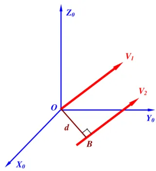
Figure 2.1 depicts two parallel vectorsv1 andv2 with the same direction and length. Thus,v1=v2 under the point vector definition, whilev1=v2 if the two vectors are considered as line vectors, because they are separated with a nonzero distanced. As a default, we say a vector is a point vector, unless it is specifically indicated as a line vector. For example, in the later analysis and applications of robotics and digital human modeling, to uniquely determine an axis for a robot link coordinate system with respect to the common base, two point vectors have to be defined: one is a 3D unit vector indicating

E.Y.L. Gu,A Journey from Robot to Digital Human, 15

Modeling and Optimization in Science and Technologies 1,

(37)

16 2 Mathematical Preliminaries

X

0

Z

0

Y

0

V

1

V

2

d

O

B

Fig. 2.1 Two parallel vectors have a common length

its direction and the other one is a 3D position vector that determines the location of the origin of that link coordinate frame with respect to the base. A 3D vector (of course, this is a point vector as default) is often denoted by a 3 by 1 column. The mathematical operations between two vectors include their addition, subtraction and multiplication. The vector multiplication has two diﬀerent categories: the dot (or inner) product and the cross (or vector) product [2, 3]. Their definitions are given as follows:

1. Dot Product – For two 3D vectors

v1= ⎛

⎝

a1

b1

c1 ⎞

⎠ and v2=

⎛

⎝

a2

b2

c2 ⎞

⎠,

v1·v2=v2·v1=v1Tv2=v2Tv1=a1a2+b1b2+c1c2, which is a scalar.

2. Cross Product – To determinev1×v2, first, let a 3 by 3 skew-symmetric matrix forv1be defined as

S(v1) =v1×= ⎛

⎝

0 −c1 b1

c1 0 −a1

−b1 a1 0

⎞

(38)

2.1 Vectors, Transformations and Spaces 17

Then,v1×v2=S(v1)·v2which is still a 3 by 1 column vector.

The major properties for the two categories of vector multiplication are outlined as follows:

1. The dot productv1·v2=v1v2cosθ, whereθis the angle between the positive directions of the two vectors, while the cross productv1×v2= v1v2sinθ, and its direction is perpendicular to both v1 and v2 and determined by the Right-Hand Rule.

2. For two non-zero vectors,v1·v2= 0 if and only ifv1⊥v2, andv1×v2= 0 if and only ifv1v2.

3. Dot product is commutable, as shown above, while the cross product is not but is skew-symmetric, i.e.,v1×v2=−v2×v1.

4. Both dot and cross products have no inverse. In other words, there is no identity vector in any of the two vector multiplication operations. 5. A successive cross product operation, in general, is not associative, i.e.,

for three arbitrary non-zero vectors, (v1×v2)×v3 = v1×(v2×v3). For instance, ifv2v3 but they both are not parallel tov1, and all the three vectors are non-zero, then, (v1×v2)×v3= 0, while v1×(v2×v3) = 0.

6. ATriple Scalar Product is defined by (v1v2v3) =v1·(v2×v3). By using

the skew-symmetric matrix for v2, it can be re-written as (v1v2v3) =

vT

1S(v2)v3. If taking the transpose, then,

(v1v2v3) =−vT3S(v2)v1=v3TS(v1)v2=v3·(v1×v2) = (v3v1v2).

Similarly,

(v1v2v3) = (v3v1v2) = (v2v3v1) =−(v1v3v2) =−(v2v1v3) =−(v3v2v1). Furthermore, if eachvi= (aibici)T fori= 1,2,3, then

(v1v2v3) = det ⎛

⎝

a1 b1 c1

a2 b2 c2

a3 b3 c3 ⎞

⎠.

Therefore, the three vectors lie on a common plane if and only if

(v1v2v3) = 0.

7. ATriple Vector Productis defined byv1×(v2×v3). Using a direct

deriva-tion, it can be proven that

v1×(v2×v3) = (v1·v3)v2−(v1·v2)v3= (vT1v3)v2−(vT1v2)v3. (2.1)

(39)

18 2 Mathematical Preliminaries

v1×(v2×v3) +v2×(v3×v1) +v3×(v1×v2)≡0.

As a numerical example, let

v1=

The triple scalar product becomes

(v3v1v2) =v3·(v1×v2) = (−4 0 2)

Thus, both approaches to evaluating the triple scalar product agree with each other.

Furthermore, the triple vector product can be calculated by

v3×(v1×v2) =S(v3)(v1×v2) =

It can also be evaluated by

v3×(v1×v2) = (vT3v2)v1−(v3Tv1)v2= 6

Therefore, the two diﬀerent ways for calculating the triple vector product match their answers with each other, too.

Both the two vector multiplication categories are very useful, especially in robotics and digital human modeling. In physics, the work W done by a force vectorf that drives an object along a vectorscan be evaluated by the dot-productW =f ·s =fT_s_{. If a force vector}_f _{is acting on an object for}

(40)

2.1 Vectors, Transformations and Spaces 19

After the vector definitions and operations are reviewed, we now turn our attention to 3D transformations. A linear transformation in vector space is a linear mappingT : Rn_→_Rm_{, which can be represented by an}_m_by_n_matrix.

In robotics, since rotation is one of the most frequently used operations, let us take a 3 by 3 rotation matrix as a typical example to introduce the 3D linear transformation.

Because a vector to be rotated should keep its length unchanged, a rotation matrix must be a length-preserved transformation [4, 5]. A 3 by 3 orthogo-nal matrix that is a member of the following Special Orthogonal Groupcan perfectly play such a unique role in performing a rotation as well as in rep-resenting the orientation of a coordinate frame:

SO(3) =

R∈R3×3_|_RRT ₌_I _{and det(}_R_{) = +1}

.

Based on the definition, a 3 by 3 rotation matrix R ∈ SO(3) has the following major properties and applications:

1. R−1₌_RT _.

2. If a rotation matrixRis also symmetric, thenR2₌_RRT ₌_I_{. This means}

that a vector rotated by such a symmetricRsuccessively twice will return to itself. This also implies that a symmetric rotation matrix acts either a 00_{rotation or a 180}0_{rotation, and nothing but these two cases.}

3. One of the three eigenvalues for a rotation matrix R ∈ SO(3) must be +1, and the other two are either both real or complex-conjugate such that their product must be +1. This means that there exists an eigenvector

x∈R3_{such that}_Rx₌_x_.

4. A 3 by 3 rotation matrixRi

bcan be used to uniquely represent, in addition

to vector or frame rotations, the orientation of a coordinate frameiwith respect to a reference frameb. Namely, each column of the rotation matrix

Ri

b is a unit vector, and they represent, respectively in order, thex-axis,

they-axis and thez-axis of frame iwith respect to frameb.

5. If a vector vi is currently projected on frame i and we want to know

the same vector but projected on frame b, then vb = Ribvi if Rbi is the

orientation of frameiwith respect to frameb.

The Lie groupSO(3) is also a 3D topological space, which can be spanned by the basis of three elementary rotations:R(x, α) that rotates a frame about its x-axis by an angle α, R(y, β) that rotates about the y-axis by β, and

R(z, γ) to rotate about the z-axis by γ. The detailed equations of the basis are given as follows:

R(x, α) = ⎛

⎝

1 0 0

0 cα −sα

0 sα cα

⎞

⎠, R(y, β) = ⎛

⎝

cβ 0 sβ

0 1 0

−sβ 0 cβ

⎞

A Journey from Robot to Digital Human

Modeling and Optimization in Science and Technologies

A Journey from

Robot to

Digital Human

Edward Y.L. Gu

Mathematical Principles and

Applications with MATLAB Programming

Modeling and Optimization in Science

and Technologies

Volume 1

About This Series

Edward Y.L. Gu

A Journey from Robot to

Digital Human

Mathematical Principles and Applications with

MATLAB Programming

Preface

Contents

List of Figures

Chapter 1

Introduction to Robotics and Digital

Human Modeling

1.1

Robotics Evolution: The Past, Today and

Tomorrow

Teleoperators

(TOP)

Numerical

Controlled Milling

Machines

M

Intelligent

Service Robots

Industrial

Robots

Digital Human

Physical Models

& Motions

Humanoid

Robots

Mobile

Robots

Field

Robots

Non-Robotic

Systems

Control App.

Robotics

Research

Flexible

Automation

Walking

Robots

Smart Digital

Human

Integration

Home

Robots

1.2

Digital Human Modeling: History, Achievements

and New Challenges

1.3

A Journey from Robot Analysis to Digital Human

Modeling

References

Chapter 2

Mathematical Preliminaries

2.1

Vectors, Transformations and Spaces

X

Z

Y

V

V

d

O

B