The Effect of Minimum Wages on
Youth Employment in Canada
A Panel Study
Terence Yuen
a b s t r a c t
Previous U.S. panel estimates of minimum wage effects have been criti-cized on the grounds that their identification rests on comparisons of ‘‘low-wage’’ and ‘‘high-wage’’ workers. Using Canadian panel data for 1988–90, I compare estimates based on the traditional U.S. methodology with those based on samples of ‘‘low-wage’’ workers exclusively. The re-sults would appear to vindicate the critics: The minimum wage effect from the latter approach is virtually zero. Yet, estimates from different subgroups of low-wage workers indicate that there is a significant disem-ployment effect for those with longer low-wage emdisem-ployment histories. This highlights the heterogeneity within low-wage workers and the importance of carefully defining the target group not solely based on workers’ wages.
I. Introduction
In the neoclassical framework, an increase in the minimum wage re-duces employment for those workers with wages at or near the minimum level. Most of the early U.S. and Canadian empirical evidence is consistent with this ‘‘standard prediction’’ of a negative employment effect (Brown 1988; Swidinsky 1980; Schaafsma and Walsh 1983). In general, aggregate studies using time series data from the 1970s and early 1980s conclude that a 10 percent increase in minimum wage decreases the
Terence Yuen is a senior analyst at the Bank of Canada. The views expressed herein are solely those of the author and should not be attributed to the Bank of Canada. The author is very grateful to Mi-chael Baker and Dwayne Benjamin for their continued guidance in conducting this study. He also thanks Irene Ip, Felice Martinello, an anonymous referee, and seminar participants at the University of Toronto, and the 1996 Canadian Economics Association Meetings for helpful comments. The Canadian International Labour Network provided financial support for this research. The data used in this article can be obtained beginning February, 2004 through January 2007 from the author at the Bank of Can-ada, 234 Wellington, Ottawa, Ontario, K1A 0G9.
[Submitted June 1998; accepted February 2002]
ISSN 022-166X2003 by the Board of Regents of the University of Wisconsin System
teenage employment by 1 to 3 percent1(Brown 1988). The validity of the time-series
evidence, however, has been called into question. A number of studies in the early 1990s (Grenier and Se´guin 1991; Wellington 1991; Card 1992a and 1992b; Katz and Krueger 1992; Card and Krueger 1994; Machin and Manning 1994) suggest that the employment effect of the minimum wage is insignificant or perhaps marginally positive.2
A number of attempts have been made to bring these divergent results into line.3
One strand of the reconciliation examines workers’ employment patterns before and after an increase in the minimum wage using individual-level panel data. Linneman (1982) is an early study adopting this approach. Using a similar framework, Currie and Fallick (1996) examine increases in the U.S. minimum wage in 1980 and 1981. They find that young people who are ‘‘bound’’ by the two minimum wage changes (that is, their current wage rate is between the old and new minimum) are 3 percent less likely to be employed in the following year.
Both the Currie and Fallick results and those in Linneman’s study have been criti-cized on the grounds that panel estimates of minimum wage effects are biased due to the lack of a suitable control group. Since the minimum wage in the United States is under the jurisdiction of the federal government, all workers in the covered sectors with wage rates near the minimum are affected simultaneously by a change in the legislation. Therefore, there are few candidates to serve as a control for unrelated concurrent changes in labor market outcomes; typically the control group is mainly higher wage workers.4In other words, the panel results are based on a comparison
of ‘‘low-wage’’ and ‘‘high-wage’’ individuals.5It is possible therefore, that the panel
estimates partly capture any differences in employment stability between the two wage groups. For instance, Card and Krueger (1995a, p. 224) observe:
High-wage workers provide a poor comparison group for studying the employ-ment histories of low-wage workers. The insight from the ‘‘natural experi-ments’’ approach to empirical research is that it is crucial to have a control group representing the experiences that the affected group of workers would have had in the absence of the minimum wage increase.
1. The effects for young adults are often smaller and insignificant, reflecting their smaller representation in the minimum wage population.
Yuen 649
Obtaining an appropriate control group becomes the central challenge for panel studies of minimum wage. Perhaps the most convincing control group that has been used in U.S. studies is low-wage workers in the uncovered sectors. For example, Ashenfelter and Card (1981) re-examine Linneman’s analysis, comparing low-wage workers in the covered sectors to those in uncovered sectors. As reported in Card and Krueger (1995a), their results indicate that both groups of low-wage workers share similar employment experiences following the minimum wage increases in 1974 and 1975. This suggests that the significant disemployment effect of the mini-mum wage found in Linneman’s study is a result of the heterogeneity between high-wage and low-high-wage individuals. Canada, arguably, provides an even better environ-ment in which to address this issue. In contrast to the United States, the minimum wage in Canada is under provincial jurisdiction. Therefore, for an increase in the minimum wage in a given province, low-wage workers in other provinces can serve as the control group. In this case, the minimum wage effect is identified by variation between two groups of low-wage individuals with comparable experience.
Using data from the Labour Market Activity Survey, I examine the effects of provin-cial minimum wage increases in Canada between 1988 and 1990. Over the sample period, there were a total of 19 separate changes in minimum wages across ten prov-inces. I begin by adopting the U.S. panel methodology: that is, including high-wage individuals in the control group. Fixed effect estimates of the effect of the minimum wage on employment probability are negative and significant for both teens and young adults. This result is consistent with other U.S. panel estimates of minimum wage effect. I next replicate the analysis limiting the control group to low-wage workers in provinces with no minimum wage change. The resulting estimates of the minimum wage effect are insignificant and virtually zero. The difference in the results across these two methods appears to validate the criticism of past panel studies of minimum wages. The negative and significant estimates from the first method are driven by differences in employment stability between high-wage and low-wage workers.
This paper proceeds as follows: Section II describes the key aspects of the longitu-dinal data set. Because no micropanel study has previously been conducted for Can-ada, Section IIIA replicates the U.S. panel studies by including high-wage individu-als. In Section IIIB, I limit my sample to only low-wage observations in order to determine whether the results are sensitive to the definition of the control group. Section IV contains some concluding remarks.
II. Data
The Labour Market Activity Survey (LMAS) is a longitudinal labor market data set which is a representative of the Canadian population.6 Individuals
are initially (1988) sampled through an addendum to the Labour Force Survey. They are then recontacted annually (1989 and 1990) and questioned about their labor mar-ket behavior in the intervening period. In addition to general demographic informa-tion, the survey contains detailed employment informainforma-tion, such as weekly employ-ment status and the beginning and end dates of different nonemployemploy-ment spells. Since the primary objective of this paper is to retrieve panel estimates of minimum wage effects on youth employment, only people between ages 16 and 24 in 1988 are included in my sample.7
The LMAS provides weekly employment status for each individual and it is possi-ble to construct a weekly panel on the labor market activity of each individual every year. However, control variables, such as provincial unemployment rate and con-sumer price index, are provided at most on a monthly basis, and changes in the main variable of interest, the minimum wage, are even less frequent. I therefore work with quarterly data that capture each individual’s employment status8 at the middle of
each quarter;9that is, at most 12 observations for each individual during the
three-year sample period. Also, I exclude any individual who moves to the Yukon and Northwest Territories over the sample period because a complete series of all the control variables is not available for these areas.
I focus on the effect of the minimum wage on the transition from employment to nonemployment. Therefore, I confine my sample to those who are employed with a positive wage rate in a given quarter. In the LMAS, an hourly wage rate may not be directly reported by the individual. Any wage of salary that is not reported on an hourly basis is converted to an hourly equivalent rate as the usual wage or salary (for example, daily, weekly or monthly) divided by the total hours worked. Observa-tions with hourly wages lower than $2 or higher than $50 are excluded because they likely result from measurement error, especially for young adults. I also note that
6. Individuals living in the Yukon and Northwest Territories are not sampled in the LMAS.
7. Because my sample ‘‘ages’’ over time, these individuals will be 18–26 by the last year of the panel. 8. The LMAS attempts to decompose nonemployment into three states: Unemployment with job search, unemployment without job search, and not in the labor force. As pointed out by Jones and Riddell (1994), there are problems with this filter of the data. It may lead to biased measurement of the incidence and duration of nonemployment when there are only two meaningful nonemployment, states. However, the LMAS longitudinal file provides a perfect forum for my analysis that only focuses on movements between employment and nonemployment in a two-state framework.
Yuen 651
Table 1
Summary Statistics for the Pooled Cross Sections 1988–90
Teens Young Adults
Number of observations 28,849 42,153
Number of individuals 4,379 5,000
Male ratio (percent) 52.27 50.14
Marriage rate in 1990 (percent) 6.86 47.71
Education in 1990 (percent)
0–8 years of education 2.57 6.42
Some secondary education 49.14 15.60
Graduated from high school 21.43 30.28
Some post-secondary 19.14 19.27
Post-secondary diploma 4.29 11.01
University degree 0.29 10.99
Trade certificate or diploma 3.14 7.34
Province (percent)
Newfoundland 6.04 5.65
P.E.I. 2.66 3.10
Nova Scotia 5.90 7.34
New Brunswick 8.73 8.21
Quebec 13.43 16.91
Ontario 22.44 21.50
Manitoba 7.65 7.07
Saskatchewan 8.95 8.39
Alberta 14.02 13.47
British Columbia 10.19 8.38
Average total employment periods 6.59 8.44
Average wage ($) 6.78 9.22
Notes: Data are from the LMAS 1998–90 Job File. Teens are defined as individuals aged 16–19 in 1988. Young adults are individuals aged 20–24 in 1988.
individuals with multiple jobs may have more than one hourly wage rate for a given period. Different weighted averages of the wage rates for different jobs can be used as the final measure of individual wage at a given time. It is reasonable to assume that the likelihood of losing a job decreases as the wage rate increases. Therefore, for those who hold more than one job in a period, what I am really interested in is to see whether they will lose their highest paid jobs and become unemployed as a result of a minimum wage increase. Taking the highest among all the wage rates as the final measure seems to be more appropriate.10
My full sample contains 71,002 observations on 9,379 individuals. There are 4,379
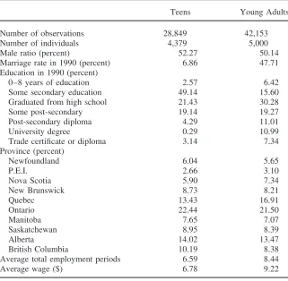
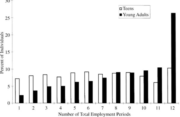
Figure 1
Distribution of Total Employment Periods by Age
teenagers between the ages of 16 to 19 (in 1988), while the remaining 5,000 are young adults of ages 20 to 24. The percentage male are 52.3 and 50.1 for teenagers and young adults respectively. Descriptive statistics for the pooled cross section (1988 to 1990) are presented in Table 1. Not surprisingly, the marriage rate and education level of young adults are significantly higher that teens. Young adults work longer hours at higher wages. The mean wages are 6.78 and 9.22 for the teens and young adults respectively. In addition, the average employment history of young adults is almost half a year longer than for teens. Young adults have 8.4 quarters employed throughout the three-year sample period while the mean is only 6.6 for teens. As shown in Figure 1, the sample distribution of the number of total employment periods for young adults is heavily skewed to the right. More than 25 percent of the young adults are employed in all 12 quarters between 1988 and 1990.
Yuen
653
Table 2
Percentage of Individuals ‘‘At-Risk’’ by Province
1988 1989 1990
1st 2nd 3rd 4th 1st 2nd 3rd 4th 1st 2nd 3rd 4th
Quarter Quarter Quarter Quarter Quarter Quarter Quarter Quarter Quarter Quarter Quarter Quarter
Newfoundland T 4.00
Y 0.65
P.E.I. T 10.53 3.85
Y 2.86 4.49
Nova Scotia T 17.95
Y 7.72
New Brunswick T 10.34 9.52 6.89
Y 2.87 2.17 2.72
Quebec T 12.97 7.33 11.11
Y 1.98 2.33 3.05
Ontario T 9.57 4.93 12.16
Y 1.92 1.84 3.01
Manitoba T
Y
Saskatchewan T 13.55 4.66
Y 2.13 1.04
Alberta T 13.03
Y 1.62
British Columbia T 17.55 6.71 2.82
Y 2.91 3.19 1.03
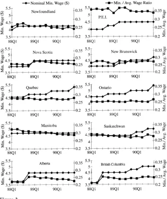
As noted above, over the three-year sample period there were 19 minimum wage changes in different provinces. Figure 2 shows at least one minimum wage increase in all provinces, except Manitoba. We might expect the nominal minimum wage to trend upward over the period, as provincial governments may adjust the level in order to match the inflation rate. On the other hand, there is no common pattern in the trends of the relative minimum wage, measured as the ratio of the nominal mini-mum wage to the average provincial manufacturing wage11(MinW/AvgW). This is
in part due to the fact that there have been distinct minimum wage policies in the provinces over the period.12As expected, provinces like Ontario and Quebec, which
revised their minimum wages yearly during the sample period, have a more stable pattern in the relative minimum wage.
III. Empirical Evidence
A. The ‘‘Traditional’’ Approach—All Employed Individuals
If minimum wages and employment are negatively correlated, an increase in mini-mum wage will increase the likelihood of those currently employed being laid off or unable to find new jobs through regular turnover in the next period. In other words, the probability of shifting from employment to nonemployment increases. Given that an individual is employed int⫺1, the probability of being employed in the next period is modeled as a function of a set of control variables and the variable measuring exposure to the minimum wage increase.
(1) Pr(Sj
i,t⫽1|Sji,t⫺1⫽1)⫽f(AtRiskji,t,Iji,t,Vjt,Dp,Dy,Ds)⫹εji,t Sj
i,tis the employment status of individualiliving in provincejat timet. The binary dependent variable (Ej wage rate of individualiat period t⫺1 is between the old minimum (MinWj
t⫺1)
and the new minimum (MinWjt) when there is a minimum wage increase in province j at t, and ⫽ 0 otherwise.14 Thus, individuals with wages outside this range
([MinWj
t⫺1,MinWjt]), as well as all workers in other provinces with no minimum wage changes, are used as the control group for other changes in the labor market. This ‘‘traditional’’ approach has been adopted in other U.S. panel studies, such as Currie and Fallick (1996).15
11. It is the provincial average manufacturing wage including overtime.
12. Besides minimum wage policy,AvgWdiffers across provinces. This may also lead to difference in (MinW/AvgW). For example, the exceptionally high relative minimum wage in P.E.I. is due to its relatively low manufacturing wage compared with other provinces.
13. Since employment status before 1998 is not reported in the survey, the sample for empirical estimations begins in the second quarter of 1998. As a result, 5,759 observations are excluded from the full sample. 14.AtRiskj
i,t⫽0 if (i) there is no minimum wage in provincejattor (ii) the wage rate of individuali
is below the old minimum (MinWj
t⫺1) or above the new minimum (MinW
j t).
Yuen 655
The demographic information for individuali(marital status, education level, and gender) is represented byIj
i,t. One point worth mentioning is that labor force
experi-ence or potential experiexperi-ence is not included as one of the control variables. Because the LMAS records age and education level by categories, it is not possible to infer the exact age and years of schooling of each individual from this classification. Vj
trepresents the economic environment of provincejat timet, which includes the real GDP, the level as well as the change in unemployment rate of prime-age males (aged 25–54) between periodt⫺ 1 and t.Dpare provincial dummy variables to capture the provincial fixed effects. Dummy variables,DyandDs, are year and season effects respectively. Detailed descriptions of each group of independent variables are given in Table 3.
A set of estimates of the linear probability model given in Equation 1 is reported in Table 4. Starting with the OLS estimates, the coefficient onAtRiski,tis negative and statistically significant16for both teens and young adults. On average, ‘‘at-risk’’
teenagers are 7 percent less likely to be reemployed after an 8.4 percent17increase
in minimum wage. The impact is even greater on young adults at 14.8 percent.18
The OLS estimates are subject to the same criticism leveled at the other panel studies of minimum wage. The control group consists primarily of high-wage work-ers. If high-wage workers are ‘‘better’’ than low-wage workers in some unobserved quality that has a positive effect on employment and earnings, the results from the OLS estimation are biased. More precisely, the estimates of the minimum wage effects also capture these differences between high and low-wage workers. In order to control for the unobserved heterogeneity between the two wage groups, I reesti-mate Equation 1 using a fixed effect (FE) model. To ensure that there is sufficient variation in the explanatory variables, only individuals with three or more observa-tions are included in my sample for this part of the analysis.19Results are shown in
the second and fifth columns of Table 4. For both age groups, the FE estimates are still negative and statistically significant, but their magnitude is slightly less than OLS estimates. Although the differences are not substantial, there is indeed some indication that the unobserved heterogeneity across individuals is correlated with inclusion in the ‘‘at-risk’’ set.20The orthogonality of the unobserved heterogeneity
and the regressors can be formally tested by the Hausman specification test. The random effect estimates for comparison to the fixed effect estimates are reported in Columns 3 and 6. At 5 percent confidence level, the test21rejects the hypothesis of
the results (not reported) are not particularly informative because of the very small number of ‘‘at-risk’’ individuals in many provinces.
16. Standard errors in all OLS and FE models have been corrected by the White (1980) procedure. 17. This is the average percent increase of all 19 provincial minimum wage changes weighted by the number of ‘‘at risk’’ individuals in each change.
18. The weighted average percent increase in the minimum wage for young adults is 7.7 percent. Although both teens and young adults are affected by the same minimum wage changes, the weighted average percent increase is different for each age group. This is because the number of ‘‘at-risk’’ teens is different from the number of ‘‘at-risk’’ young adults.
19. As a result, 1,605 observations are dropped from the original sample.
Figure 2
Minimum Wages by Province
Yuen 657
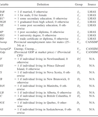
Table 3
Description of Control Variables, Xi,t
Variable Definition Group Source
MAR ⫽1 if married, 0 otherwise Ii,t LMAS
SEX ⫽1 for male, 0 for female Ii,t LMAS
SECa
⫽1 some secondary education. 0 otherwise Ii,t LMAS HIGH ⫽1 graduated from high school, 0 otherwise Ii,t LMAS PSE ⫽1 some post secondary education, 0 oth- Ii,t LMAS
erwise
DIP ⫽1 post secondary diploma, 0 otherwise Ii,t LMAS DEG ⫽1 university degree, 0 otherwise Ii,t LMAS TRD ⫽1 trade certificate or diploma, 0 otherwise Ii,t LMAS Unemp Provincial unemployment rates for males (25– Vj,t CANSIMb
54) att
UnempGP Unempt–Unempt⫺1 Vj,t CANSIM
RGdp (Provincial GDP at market price) / (Provincial Vj,t CANSIM CPI)c
NF ⫽1 if individual living in Newfoundland, 0 Dd
p N/A
otherwise
PEI ⫽1 if individual living in Prince Edward Dp N/A Island, 0 otherwise
NS ⫽1 if individual living in Nova Scotia, 0 oth- Dp N/A erwise
NB ⫽1 if individual living in New Brunswick, 0 Dp N/A otherwise
MAN ⫽1 if individual living in Manitoba, 0 oth- Dp N/A erwise
ALB ⫽1 if individual living in Alberta, 0 otherwise Dp N/A BC ⫽1 if individual living in British Columbia, 0 Dp N/A
otherwise
QUE ⫽1 if individual living in Quebec, 0 other- Dp N/A wise
SAS ⫽1 if individual living in Saskatchewan, 0 oth- Dp N/A erwise
a. Base Group has 0–8 years of education
b. Canadian Socio-Economic Information Management System c. Base year⫽1986
The
Journal
of
Human
Resources
Table 4
Estimates of the Effects of Minimum Wages on the Reemployment Probability for ‘‘At-Risk’’ Group—All Employed Individuals (standard errors in parentheses)
Teens: 16–19 Young Adults: 20–24
Fixed Random Fixed Random
Variable OLS Effects Effects OLS Effects Effects
AtRisk ⫺0.0702 ⫺0.0634 ⫺0.0644 ⫺0.1484 ⫺0.1034 ⫺0.1207
(0.020) (0.020) (0.016) (0.033) (0.031) (0.023)
SEX ⫺0.0115 ⫺0.0217 0.0091 0.0031
(0.005) (0.006) (0.003) (0.005)
MAR 0.0097 0.0053 0.0102 0.0125 ⫺0.0055 0.0123
(0.009) (0.018) (0.011) (0.003) (0.008) (0.004)
SEC 0.0146 ⫺0.0279 ⫺0.0002 0.0528 0.0200 0.0499
(0.021) (0.045) (0.023) (0.014) (0.042) (0.015)
HIGH 0.0320 ⫺0.0512 ⫺0.0020 0.0908 0.0181 0.0799
Yuen
659
PSE ⫺0.0260 ⫺0.1103 ⫺0.0664 0.0460 ⫺0.0107 0.0301
(0.022) (0.048) (0.024) (0.014) (0.045) (0.015)
DIP 0.0472 ⫺0.0166 0.0054 0.1072 0.0691 0.1013
(0.027) (0.054) (0.027) (0.014) (0.046) (0.015)
DEG ⫺0.0708 ⫺0.1384 ⫺0.1031 0.0968 0.1361 0.0973
(0.055) (0.094) (0.051) (0.014) (0.051) (0.016)
TRD 0.0477 ⫺0.0046 0.0201 ⫺0.0126 0.0428 0.0983
(0.027) (0.058) (0.030) (0.002) (0.045) (0.017)
Unemp 0.0084 0.0005 0.0041 0.0088 0.0044 0.0052
(0.004) (0.004) (0.003) (0.003) (0.002) (0.002)
UnempGp ⫺0.0118 ⫺0.0052 ⫺0.0092 ⫺0.0081 ⫺0.0082 ⫺0.0095
(0.003) (0.003) (0.002) (0.002) (0.001) (0.001)
RGdp ⫺0.00001 0.00005 ⫺0.00001 ⫺0.00009 0.0001 ⫺0.0001
(0.0001) (0.0001) (0.0001) (0.0001) (0.0001) (0.0001)
no correlation between the individual effects and other regressors for both age groups. This illustrates the problem of unobserved heterogeneity between high-wage and low-wage workers that could bias the minimum wage effect.
Another point worth mentioning is that the minimum wage effect is always greater for young adults’ employment than for teens. This may be due to the fact that the current wage rate is a noisy measure of an individual’s productivity, especially for teens. Some good quality teenage workers may be ‘‘trapped’’ in minimum wage jobs because that is where employment opportunities are (for example, in the fast food industry). The current wage rates of these teens do not necessarily reflect their potential productivity. On the other hand, given that the average young adult wage is much higher that the teenage average, young adults in the ‘‘at-risk’’ group are more likely to have really poor labor market prospects. Therefore, they may be more ‘‘vulnerable’’ to the impact of minimum wage.22
Based on the results in Table 4, the conclusion is that the minimum wage has a significant negative effect on the employment probability of the ‘‘at-risk’’ group. After controlling for the unobserved heterogeneity across individuals, ‘‘at-risk’’ teens are 6 percent less likely to be employed after an 8.4 percent increase in mini-mum wage. The impact on young adult employment is even larger at more than 10 percent.23These results are consistent with other U.S. panel studies, such as Currie
and Fallick (1996). Using a similar specification,24they find that ‘‘at-risk’’ teenagers
are 3 percent less likely to be employed as a result of a 7 percent25increase in the
U.S. federal minimum wage in 1980 and 1981. Canada would appear to share a comparable experience to the United States.
More generally, we must be careful comparing this set of results with other mini-mum wage studies. First, I am focusing on the disemployment effect on the ‘‘at-risk’’ workers who represent a very small portion of the entire youth population. In my sample, 9.5 percent of the teens and 2.4 percent of the young adults are consid-ered ‘‘at-risk.’’ Therefore, even though an increase in the minimum wage has a negative and significant impact on ‘‘at-risk’’ employment, it is very unlikely to lead to a reduction in overall youth employment. Second, following the existing literature,
22. In fact, I have replicated the analysis on adults between the ages of 25 and 34. In this case, the effect of minimum wage on the ‘‘at risk’’ group is slightly greater than for young adults (aged 20–24). The minimum wage effect on reemployment probability ranges from 10 to 12 percent. This further confirms the idea that an individual considered ‘‘at risk’’ in a group with a higher average wage is more likely to be a lower ‘‘quality’’ worker.
23. See footnote 18.
24. Instead of the dummy variableAtRiskj
i,t, they use a continuous variableWageGapi,tto control for the
effect of minimum wage.WageGapi,tis defined as the difference between the minimum wage attand the
wage rate of individualiatt⫺1 if he is considered as ‘‘at risk’’ in the minimum wage change att. WageGpi,t⫽0 otherwise. Conceptually, WageGpi,tis just a refinement ofAtRiskji,t.WageGpi,tfurther
distinguishes the ‘‘at risk’’ individuals based on the difference between their current wages and the mini-mum. I have also replicated the empirical analysis usingWageGapi,t. The results (not reported) are robust
to this change in specification. The coefficients onWageGapi,tare all significant and negative. For teens,
the estimates imply that on average the ‘‘at-risk’’ group is 4–5 percent less likely to be employed in the following year if there is a minimum wage increase. The implied effect on young adults is larger at⫺9–
⫺11 percent.
Yuen 661
the estimated minimum wage effect only refers to the transition from employment to nonemployment. Ideally, I should also look at the transition from nonemployment to employment in order to obtain a complete picture of the minimum wage effect on employment probability. However, I cannot use current wage rates to identify the nonemployed as ‘‘at-risk.’’
B. A Refinement of the Control Group–Only ‘‘Low-wage’’ Individuals
As noted above, most criticism of the ‘‘traditional’’ panel model focuses on the definition of the control group. Since the control group in the previous section is dominated by the high-wage individuals outside the ‘‘at-risk’’ range [MinWj
t⫺1, MinWjt], the coefficient onAtRiskj
i,tnot only captures the effect of minimum wages on the reemployment probability, but also any differences in employment stability between low-wage and high-wage individuals. If high-wage workers always have higher employment rates than low-wage workers, the estimates of the minimum wage effect in the previous section may be biased away from zero. One way to address this problem is to exploit the panel nature of the data and estimate a FE model, as reported in the previous section. Yet, assuming the individual effects for youth are fixed over time is subject to question. In commenting on Currie and Fallick (1996),26
Card and Kreuger (1995a, p. 228) argue:
[T]here is little reason to believe that, for the NLSY sample, the unobserved individual effects that are correlated with the base-year pay are fixed, or even approximately fixed, over time. . . . In such a sample, one would expect produc-tivity, wages, and employment rates to evolve rapidly over time, as workers move in and out of school and shop among jobs.
An alternative solution to this heterogeneity problem is to obtain a better control group. That is replacing the high-wage workers with a group of workers with wage rates comparable to the ‘‘at-risk’’ individuals but who are not affected by the increase in minimum wage. The comparison group in the analysis of the previous section consists of two different types of people: those outside the ‘‘at-risk’’ range [MinWj
t⫺1,MinWjt] in the province with an increase in the minimum, and all workers
in other provinces with no minimum wage change. In this section, I focus on the ‘‘low-wage’’ individuals from the latter group since they are potentially a good con-trol for the ‘‘at-risk’’ individuals.27They have similar wages to the ‘‘at-risk’’ workers
and therefore are more likely to have similar employment stability.
26. In addition to the basic FE model, they include a dummy variable for workers with wage rates no more than 15 cents above the minimum. Also, they decompose the control into three different groups. Their results indicate a negative minimum wage effect even after employing these different treatments for the unobserved heterogeneity.
Newfound-There are at least three ways to define a control group of low-wage workers in a province where there is no change in the minimum wage. First, we could consider a worker as low-wage if his wage rate is within a certain fixed dollar interval above the existing minimum in his province. A second definition would be to replace the fixed dollar interval by a fixed percentage interval. By these two definitions, the wage interval is insensitive to the minimum wage changes in other provinces. There-fore, instead of imposing a time invariant margin, a changing interval could be used. It could be equal to the maximum/minimum percentage or dollar change in the mini-mum wage observed concurrently in other provinces.28In the following analysis, I
simply choose a fixed dollar interval of 25 cents since two-thirds29of these increases
in the minimum wages observed in the sample period are exactly this amount.30
Formally, individuals in provincejare considered low-wage control at timet, that is,AtRiskj
i,t ⫽0, if their wages at time tare between MinWjtandMinWjt⫹ 0.25 when the minimum wage of provincejremains unchanged. It is important to note that more than 93 percent of the control group used in the previous section is ex-cluded by this definition.31A detailed decomposition of the entire sample is presented
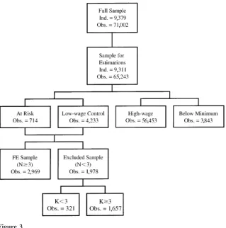
in Figure 3.
To check whether high-wage workers normally have more stable employment histories than low-wage workers, I compare the average employment rates between the two wage groups during periods with no minimum wage change. The empirical framework is similar to Equation 1. Instead of measuring the minimum wage effect, AtRiskj
i,tis replaced by the dummy variable,LowWji,t, indicating whether the
individ-ual in the provincejat timetis considered as a low-wage worker defined above.32
Conceptually,LowWj
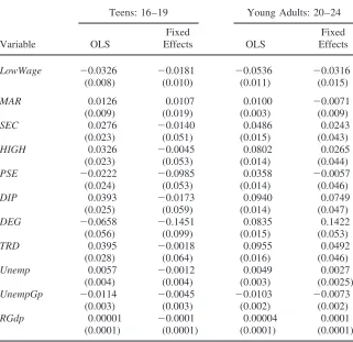
i,t will capture the employment rate differentials across wage groups. As reported in Table 5, the OLS and FE estimates ofLowWj
i,tare negative and statistically significant for both teens and young adults. Hence, high-wage workers are relatively more stable, even after controlling for workers’ unobserved quality.
As an alternative evaluation of the heterogeneity problem, Equation 1 is reesti-mated using only low-wage workers as control. The results are presented in Table 6. Again, I begin with a linear probability model estimated by OLS. For teens (Table 6A) the estimate of the minimum wage effect is negative, but virtually zero. In addition, the standard error is much greater than the estimate. For young adults (Table
land, Nova Scotia, and Prince Edward Island. Results (not reported) focusing on the Atlantic region are very similar to the main results reported in Tables 4 to 6. Furthermore, Fortin, Keil, and Symons (2001) provides some empirical evidence on the homogeneity across Canadian regions. For young men and women between 15 and 24, the factors contributing to their unemployment rates over the years 1967–91 are not regional specific.
28. Mathematically, three low-wage control definitions are: (i) MinWj
t⫺1 ⫹ a fixed amount, (ii) MinWj
t⫺1⫻(1⫹a fixed percentage change), and (iii)MinWjt⫺1⫹maximum/minimum dollar change of the minimum in other provinces orMinWj
t⫺1⫻(1⫹maximum/minimum percentage change of the min-imum).
29. 12 of 19 provincial minimum wage changes are exactly $0.25.
30. I have replicated the analysis with all three measures. The results (not reported) are similar to those reported in Table 6.
31. Figure 3 shows that 60,296 are excluded from the control.
32. That is,LowWji,t⫽1 if the worker’s wage is within 25 cents above the existing minimum wage in
Yuen 663
Figure 3
Detailed Breakdown of the Sample
Notes: K⫽Total periods of employment between 1988–90. N⫽Number of low wage employment periods be-tween 1988–90.
6B), the estimate is negative with greater precision and magnitude, but still is not significant even at 10 percent confidence level. Therefore, empirical evidence in both Tables 5 and 6 would seem to confirm the criticism of previous U.S. panel studies. The minimum wage effect is biased because of the absence of an adequate control group. Once the comparison group is restricted to low-wage individuals, there is no minimum wage effect on youth employment, even for those ‘‘at risk.’’
The purpose on focusing on low-wage workers is to eliminate the unobserved heterogeneity among workers. The treatment and the control groups are supposed to have comparable employment experience ex ante. Therefore, we would expect the results from a FE model to be very similar to the OLS. Surprisingly however, the FE model provides a very different picture. The results are reported in the second column of Table 6A and 6B. Here the estimated parameters onAtRiskj
Table 5
Differentials in the Reemployment Probability between Low-wage and High-wage Individuals (standard errors in parentheses)
Teens: 16–19 Young Adults: 20–24
Fixed Fixed
Variable OLS Effects OLS Effects
LowWage ⫺0.0326 ⫺0.0181 ⫺0.0536 ⫺0.0316
(0.008) (0.010) (0.011) (0.015)
MAR 0.0126 0.0107 0.0100 ⫺0.0071
(0.009) (0.019) (0.003) (0.009)
SEC 0.0276 ⫺0.0140 0.0486 0.0243
(0.023) (0.051) (0.015) (0.043)
HIGH 0.0326 ⫺0.0045 0.0802 0.0265
(0.023) (0.053) (0.014) (0.044)
PSE ⫺0.0222 ⫺0.0985 0.0358 ⫺0.0057
(0.024) (0.053) (0.014) (0.046)
DIP 0.0393 ⫺0.0173 0.0940 0.0749
(0.025) (0.059) (0.014) (0.047)
DEG ⫺0.0658 ⫺0.1451 0.0835 0.1422
(0.056) (0.099) (0.015) (0.053)
TRD 0.0395 ⫺0.0018 0.0955 0.0492
(0.028) (0.064) (0.016) (0.046)
Unemp 0.0057 ⫺0.0012 0.0049 0.0027
(0.004) (0.004) (0.003) (0.0025)
UnempGp ⫺0.0114 ⫺0.0045 ⫺0.0103 ⫺0.0073
(0.003) (0.003) (0.002) (0.002)
RGdp 0.00001 ⫺0.0001 0.00004 0.0001
(0.0001) (0.0001) (0.0001) (0.0001)
Notes: See notes in Table 4. ‘‘LowWage’’ is a dummy variable that takes the value 1 if the individual’s wage is within 25 cents above the existing minimum wage in provincejat timet, 0 otherwise.
Yuen
665
Table 6A
Additional Estimates of the Effects of Minimum Wages on the Re-employment Probability for the ‘‘At-Risk’’ Teens (standard errors in parentheses)
OLS OLS
OLS FE OLS Nⱖ3 vs. OLS Nⱕ3 vs.
Variable Low Wage Nⱖ3 Nⱖ3 High Wage Nⱕ3 High Wage
AtRisk ⫺0.0040 ⫺0.0969 ⫺0.0724 ⫺0.0527 0.0989 ⫺0.2424
(0.024) (0.032) (0.030) (0.026) (0.036) (0.030)
SEX 0.0020 0.0063 ⫺0.0252 0.0280 ⫺0.0246
(0.014) (0.015) (0.005) (0.025) (0.005)
MAR ⫺0.0513 ⫺0.0044 ⫺0.0428 0.0066 ⫺0.0857 0.0058
(0.033) (0.094) (0.037) (0.009) (0.058) (0.009)
SEC 0.1251 ⫺0.0734 ⫺0.0389 0.0370 0.2150 0.0376
(0.076) (0.010) (0.051) (0.024) (0.115) (0.024)
HIGH 0.1301 ⫺0.0983 ⫺0.0591 0.0356 0.2796 0.0376
(0.077) (0.113) (0.053) (0.024) (0.115) (0.024)
PSE 0.0751 ⫺0.2060 ⫺0.0886 ⫺0.0150 0.1819 ⫺0.0135
(0.077) (0.121) (0.054) (0.025) (0.115) (0.025)
DIP 0.0505 ⫺0.4049 ⫺0.1665 0.0476 0.2599 0.0479
(0.087) (0.152) (0.076) (0.026) (0.131) (0.026)
DEG ⫺0.0242 ⫺0.4767 ⫺0.2474 ⫺0.0872 ⫺0.0566 ⫺0.0837
(0.162) (0.250) (0.157) (0.059) (0.351) (0.060)
TRD 0.1292 ⫺0.2179 ⫺0.0469 0.0270 0.3246 0.0263
(0.094) (0.170) (0.077) (0.030) (0.157) (0.030)
Unemp 0.0126 ⫺0.0095 ⫺0.0026 ⫺0.0001 0.0228 0.0006
(0.011) (0.014) (0.012) (0.004) (0.018) (0.004)
UnempGp ⫺0.0062 0.0018 ⫺0.0015 ⫺0.0077 ⫺0.0058 ⫺0.0076
(0.008) (0.009) (0.009) (0.003) (0.014) (0.004)
RGdp 0.0001 0.0006 ⫺0.0003 0.0001 0.0013 0.0001
(0.0003) (0.0004) (0.0004) (0.0001) (0.001) (0.0001)
The
Journal
of
Human
Resources
Additional Estimates of the Effects of Minimum Wages on the Reemployment Probability for the ‘‘At-Risk’’ Young Adults (standard errors in parentheses)
OLS OLS
OLS FE OLS Nⱖ3 vs. OLS Nⱕ3 vs.
Variable Low Wage Nⱖ3 Nⱖ3 High Wage Nⱕ3 High Wage
AtRisk ⫺0.0504 ⫺0.1124 ⫺0.0967 ⫺0.0851 0.0257 ⫺0.3045
(0.041) (0.040) (0.048) (0.039) (0.069) (0.055)
SEX 0.0270 0.0368 0.0013 0.0523 0.0015
(0.023) (0.023) (0.003) (0.042) (0.003)
MAR ⫺0.0221 ⫺0.0322 0.0120 0.0083 ⫺0.0322 0.0084
(0.025) (0.097) (0.025) (0.003) (0.046) (0.003)
SEC 0.1165 ⫺0.0059 0.1077 0.0419 0.1950 0.0406
(0.076) (0.096) (0.089) (0.015) (0.115) (0.015)
HIGH 0.2094 ⫺0.0151 0.1366 0.0701 0.2421 0.0689
(0.071) (0.061) (0.084) (0.014) (0.113) (0.014)
PSE 0.1326 ⫺0.0360 0.0719 0.0271 0.2617 0.0268
(0.072) (0.088) (0.086) (0.014) (0.110) (0.014)
DIP 0.1195 0.1653 0.0895 0.0830 0.2508 0.0820
(0.077) (0.137) (0.089) (0.014) (0.116) (0.014)
DEG 0.2190 0.1568 0.2337 0.0710 0.2410 0.0701
(0.078) (0.119) (0.083) (0.015) (0.127) (0.015)
TRD 0.2187 ⫺0.0246 0.1426 0.0778 0.3866 0.0772
(0.086) (0.015) (0.104) (0.016) (0.130) (0.016)
Unemp ⫺0.0140 0.0030 0.0025 0.0045 ⫺0.0573 0.0042
(0.016) (0.021) (0.017) (0.003) (0.028) (0.003)
UnempGp ⫺0.0012 ⫺0.0246 ⫺0.0206 ⫺0.0083 0.0311 ⫺0.0082
(0.011) (0.015) (0.011) (0.002) (0.020) (0.002)
RGdp ⫺0.0002 0.0008 0.0001 ⫺0.0001 ⫺0.0004 ⫺0.0001
(0.001) (0.001) (0.001) (0.0001) (0.001) (0.0001)
Yuen 667
observations33are included. As a result, 40 percent34of the OLS sample is excluded.
In order to identify the effects of this sample selection, I present OLS estimates using the FE sample. The results for both age groups, reported in Column 3, are very similar to the FE estimates: The estimated minimum wage effects are negative and statistically significant. Thus the difference between the FE estimates in Column 2 and the OLS estimates in Column 3 is due to sample selection rather then hetero-geneity.
The empirical evidence thus far suggests that only low-wage workers in the FE sample are likely to be affected by the minimum wage. A natural follow-up question is how sensitive this result is to various control groups. In particular, the central issue is whether a high-wage control group would bias the minimum wage effect. In Column 4, ‘‘at-risk’’ workers in the FE sample are compared to the high-wage workers who have more than three periods of high-wage employment during the sample period. Surprisingly, for both age groups the coefficients on theAtRiskj
i,tare similar to those in Column 3 when the comparison is based on low-wage workers exclusively. There is no evidence that the inclusion of high-wage individuals bias the minimum effect on the FE sample. The key finding is that, regardless of the control groups, a minimum wage increase has an adverse impact on workers with more than three periods of low-wage employments.
I next repeat the analysis for those in the excluded sample who have less than three periods of low-wage employment. Compared with the FE sample’s results in Columns 3 and 4, Columns 5 and 6 present a very different picture. The estimated minimum wage effect for the excluded sample (Column 5) is positive and statistically significant for teens. For young adults, the estimate is less precise, but still positive. Although this somewhat surprising result is contrary to the conventional view that the minimum wage has an adverse impact on employment, it is similar to the main finding in Card and Krueger (1994 and 2000).35The minimum wage effect in the
last column becomes very negative and statistically significant for both age groups when high-wage workers serve as the control group. These divergent results clearly demonstrate the heterogeneity problem that overstates the minimum wage effect on the excluded low-wage sample.
The estimates from different subgroups of the wage sample indicate that low-wage workers are not a homogenous group. There is a significant disemployment effect on individuals with three or more low-wage employments (FE sample), but not on the complementary group (excluded sample). Descriptive statistics show that these low-wage groups differ in two main areas. First, individuals in the excluded sample have a shorter average employment history. Including all low and high-wage employments, they are employed for only 5.7 quarters throughout the three-year sample period, while the mean in the FE sample is 8.1 quarters. Second, they appear to be transitory low-wage workers. Only one in three of their employments is consid-ered low-wage. To address the question of why the minimum wage effect is corre-lated with the number of low-wage employment periods, I further explore the charac-teristics of the excluded individuals who may be subdivided into the following two groups:
Figure 4
Distribution of Low Wage Employment Periods across Time
Notes: K⫽Total periods of employment between 1988–90. The samples are defined in the notes in Fig-ure 3.
1. Individuals with Low-wage Employments⬍3 and Total Employments⬍3
One reason workers will have fewer than three periods of low-wage employment is that they are employed in only one or two quarters throughout the entire sample period. A prominent feature of this group is that they have an extremely high job separation rate. On average, given that they are employed in the present period, the probability of being nonemployed in the next period is 70 percent. Considering that my sample only consists of young people between the ages of 16 and 24, there are at least two hypotheses to account for short employment histories combined with high separation rates. One is that this group is comprised of low-wage workers with extremely poor labor market prospects. Alternatively, this group could be full-time students who only work in low-paid jobs during the summer. One way to distinguish these two hypotheses is by looking at the distribution of their employment periods. We would expect the employment of those in the former category to be evenly distributed throughout the sample period, and a strong seasonal pattern for the latter. As shown in Figure 4. three large spikes occur in the third quarter of each year. This supports the hypothesis that this group of low-wage individuals with extremely short employment histories is dominated by summer job workers.36 Therefore, an
increase in the minimum wage is likely to have little impact on their voluntary sum-mer job separations.
Yuen 669
Figure 5
Distribution of Percentage of Individuals with Low-Wage Employments
Notes: See notes in Figure 4.
2. Individuals with Low-wage Employments⬍3 but Total Employmentsⱖ3
As shown in Figure 3, most of the individuals excluded from the FE sample have at least three periods of employment, but only one or two of them are considered to be low-wage. The distribution of the percentage of low-wage employment for these workers is presented in Figure 5. On average, only one in five of their employ-ment periods is defined as low-wage. In contrast, individuals in the FE sample have three in five of their employment periods defined as low-wage. Intuitively, the proba-bility of individuals being ‘‘real’’ low-wage workers should be positively correlated with their percentage of low-wage employment. If only one in ten of an individual’s employment periods is low-wage, it is unlikely that he is a ‘‘real low-wage worker.’’ Instead he is likely a high-wage worker who works temporarily in some low-paid jobs. This suggests that the current wage rate may provide a noisy measure of an individual’s permanent marginal product. For example, an individual may be in the low-wage group transitorily because of a negative shock to his wage. In addition, a transitory period of low-wage employment at the early stage of an individual’s employment history may be due to summer jobs. Approximately 50 percent of the low-wage employments for this group are in the first two periods of the workers’ employment history. In addition to having a lower percentage of low-wage employ-ment, these workers are also 5 percent less likely to be employed in below minimum wage jobs. Finally, their average earnings in high-wage employments are $0.5 higher than in the FE sample. All these observations suggest that the minimum wage might have a smaller impact on this group of effectively ‘‘high-wage’’ individuals.
been overlooked in the academic literature. Most previous studies use current wage rates to identify low-wage workers as those who are the most likely affected by the change in minimum wage policy. The preceding analysis indicates that relying on current wage rates to make the identification may be insufficient. For individuals who have extremely limited low-wage employment histories, current wages may underestimate their marginal products. A close examination of the ‘‘transitory’’ wage workers in my sample reveals that they are mainly students working in low-paid jobs during the summer, or ‘‘high-wage’’ workers temporarily trapped in low-wage positions. In terms of the target group in a supply-and-demand frame-work, they are less likely to be affected by the minimum wage.
IV. Conclusion
Previous U.S. panel estimates of minimum wage effects have been criticized on the grounds that they are based on comparisons between low-wage and high-wage workers. As a result, the estimated disemployment effect may be driven by the difference in employment stability between the two groups. This article uti-lizes Canadian panel data for the period 1988–90 to evaluate this criticism. When high-wage workers are included in the control group, changes in the minimum wage have a strong negative impact on low-wage employment. This result is consistent with other U.S. panel studies of the minimum wage. However, the estimated mini-mum wage effect becomes insignificant once the control group is limited to low-wage workers in provinces with no minimum low-wage change.
At first glance, these results support the argument that the minimum wage effect is biased because of the inclusion of high-wage workers. A further exploration of the low-wage workers reveals that it is more than an issue of selecting a plausible control group. Defining the affected group is equally important in identifying the minimum effect on youth employment. The seemingly homogeneous group of low-wage workers can be divided into ‘‘transitory’’ and ‘‘permanent’’ low-low-wage workers based on their low-wage employment histories. An increase in the minimum wage displays opposite effects on these two groups. It has a significant disemployment effect on the ‘‘permanent’’ low-wage workers who have more than three quarters of low-wage employment throughout the sample period. A minimum wage increase of 8.4 percent leads to a 7 percent decrease in teens’ employment. The effect on young adults is even greater at 10 percent. More important, these results are robust to various control groups including high-wage workers. For ‘‘transitory’’ low-wage workers, who have less than three quarters of low-wage employment throughout the sample period, the effects of the minimum wage are virtually zero. Furthermore, transitory low-wage employments are mainly unstable positions, such as summer jobs. Therefore, using high-wage workers as the control group poses a serious prob-lem. It biases the minimum wage effect away from zero.
Yuen 671
words, when the treatment group is defined appropriately, the standard ‘‘textbook prediction’’ of a negative employment effect can still be retrieved.
References
Ashenfelter, Orley, and David Card. 1981. ‘‘Using Longitudinal Data to Estimate the Em-ployment Effects of the Minimum Wage.’’ Discussion Paper no. 98. London: London School of Economics.
Baker, Michael, Dwayne Benjamin, and Shutchita Stanger. 1999. ‘‘The Highs and Lows of the Minimum Wage Effect: A Time-Series Cross-Section Study of the Canadian Law’’ Journal of Labor Economics 17(2):318–50.
Brown, Charles. 1988. ‘‘Minimum Wage Laws: Are They Overrated?’’ Journal of Eco-nomic Perspectives 2(3):133–46.
Brown, Charles, Curtis Gilroy, and Andrew Kohen. 1982. ‘‘The Effect of the Minimum Wage on Employment and Unemployment.’’ Journal of Economic Literature 20(2):487– 528.
Burkhauser, Richard V., Kenneth A. Couch, and David C. Wittenburg. 2001. ‘‘A Reassess-ment of the New Economy of the Minimum Wage Literature with Monthly Data from the Current Population Survey.’’ Journal of Labor Economics 18(4):653–80.
Card, David. 1992a. ‘‘Using Regional Variation in Wages to Measure the Effects of the Federal Minimum Wage.’’ Industrial and Labour Relations Review 46(1):22–27. ———. 1992b. ‘‘Do Minimum Wages Reduce Employment? A Case Study of California,
1987-1989.’’ Industrial and Labour Relations Review 46(1):35–54.
Card, David, and Alan B. Krueger. 1994. ‘‘Minimum Wages and Employment: A Case Study of the Fast-Food Industry in New Jersey and Pennsylvania.’’ American Economic Review 84(4):772–93.
———. 1995a. Myth and Measurement: The New Economics of the Minimum Wage. Princeton: Princeton University Press.
———. 1995b. ‘‘Time-Series Minimum-Wage Studies: A Meta-Analysis.’’ American Eco-nomic Review 85(2):238–43.
———. 2000. ‘‘Minimum Wages and Employment: A Case study of the Fast-Food Indus-try in New Jersey and Pennsylvania: Reply.’’ American Economic Review 90(5):1397– 1420.
Currie, Janet, and Bruce C. Fallick. 1996. ‘‘The Minimum Wage and the Employment of Youth: Evidence from the NLSY.’’ Journal of Human Resources 31(2):404–28. Deere, Donald, Kevin M. Murphy, and Finis Welch. ‘‘Reexamining Methods of Estimating
Minimum-Wage Effects: Employment and the 1990-1991 Minimum-Wage Hike.’’ Amer-ican Economic Review 85(2):232–37.
Fortin, Pierre, Manfred Keil, and James Symons. 2001. ‘‘The Sources of Unemployment in Canada, 1967–91; Evidence from a Panel of Regions and Demographic Groups.’’ Ox-ford Economic Papers 53(1):67–93.
Grenier, Gilles, and Marc Se´guin. 1991. ‘‘L’incidence du salaire minimum sur le marche´ du travail des adolescents au Canada: Une reconside´ration des re´sultats empiriques.’’ L’Actualite´ e´conomique 67(2):123–43.
Jones, Stephen R. G., and Craig W. Riddell. 1995. ‘‘The Measurement of Labor Force Dy-namics with Longitudinal Data: The Labour Market Activity Survey Filter.’’ Journal of Labor Economics 13(2):351–85.
Labour Canada. 1989-93. Labour Standards Legislation in Canada. Ottawa: Supply and Ser-vices Canada. Occasional.
Linneman, Peter. 1982. ‘‘The Economic Impacts of Minimum Wage Laws: A New Look at an Old Question.’’ Journal of Political Economy 90(3):443–69.
Machin, Stephen, and Alan Manning. 1994. ‘‘The Effects of the Minimum Wages on Wage Dispersion and Employment: Evidence from the U.K. Wage Councils.’’ Industrial and Labor Relations Review 47(2):319–29.
Neumark, David, and William Wascher. ‘‘Employment Effects of Minimum and Submini-mum Wages: Panel Data on State MiniSubmini-mum Wage Laws.’’ Industrial and Labour Rela-tions Review 46(1):55–81.
———. 2000. ‘‘Minimum Wages and Employment: A Case study of the Fast-Food Indus-try in New Jersey and Pennsylvania: Comment.’’ American Economic Review 90(5): 1362–96.
Schaafsma, Joseph, and William D. Walsh. 1983. ‘‘Employment and Labour Supply Ef-fects of the Minimum Wage: Some Pooled Time-Series Estimates from Canadian Provin-cial Data.’’ Canadian Journal of Economics 16(1):86–97.
Swidinsky, Robert. 1980. ‘‘Minimum Wages and Teenage Unemployment.’’ Canadian Jour-nal of Economics 13(1):158–71.
Wellington, Alison J. 1991. ‘‘Effects of the Minimum Wage on the Employment Status of Youths, an Update.’’ Journal of Human Resources 26(1):27–46.