www.elsevier.nlrlocatereconbase
Intersectoral labour reallocations and
unemployment in Italy
Paolo Garonna
a,b,), Francesca G.M. Sica
c,1a ( )
Statistical DiÕision of the United Nations ECE , 1202 GeneÕa, Switzerland
b
UniÕersity of Padua, Padua, Italy
c
Department of Macroeconomics Analysis, Labour Market Unit, Institute for Studies and Economic
( )
Analyses ISAE , Rome, Italy
Received 5 August 1997; accepted 11 April 2000
Abstract
The Italian labour market, like most European labour markets and unlike the US, shows a greater cyclical sensitivity of the service sector with respect to manufacturing and firing costs higher than hiring costs. This accounts for the negative relationship between sectoral employment shifts and Italian unemployment in the post-war period and, correspondingly, for the pro-cyclical pattern of the Lilien index, in contrast with the US experience.
By applying the Lilien index to the Italian context, this paper analyses the relative importance of sectoral regional and national factors in the explanation of changes in industrial structure, and their impact on unemployment. The econometric exercise illustrates that, given the structural features of the Italian labour market, the decline in intersectoral and interregional labour reallocations has significantly contributed to the increase of unemployment in Italy. New hires, the pull of new sectors, sectoral shifts and regional mobility can keep unemployment down, while at the same time maintaining some of the
Ž .
structural features of the AEuropean modelB high employment security and stability .
q2000 Elsevier Science B.V. All rights reserved.
JEL classification: E24; J6
Keywords: Unemployment; Intersectoral shifts; Interregional shifts
)Corresponding author. Statistical Division of the United Nations ECE , 1202 Geneva, Switzer-Ž .
land. Tel.:q41-22-917-4144; fax:q41-22-917-0040.
Ž . Ž .
E-mail addresses: [email protected] P. Garonna , [email protected] F.G.M. Sica .
1
Tel.:q39-6-4448-2347; fax:q39-6-4448-2219
0927-5371r00r$ - see front matterq2000 Elsevier Science B.V. All rights reserved.
Ž .
1. Introduction
The Italian labour market is undergoing a profound transformation in its capacity to respond to and accommodate structural change.
Ž .
In the post-war period, the two major waves of a rapid industrialisation, Ž . accompanied by massive agricultural exodus in the 1950s and 1960s, and b tertiarization accompanied by a fundamental restructuring of mass manufacturing in the 1970s and 1980s were supported by particular mechanisms of labour flexibility derived from specific traditional and institutional arrangements. The ensuing responsiveness permitted a substantial increase in aggregate employment consistent with productivity growth and competitiveness.
In the early 1990s, however, a structural breakdown took place in the flexibility patterns of the Italian labour market. Services and the small firms sectors were hit by an unprecedented structural shock, which has not yet been matched by an appropriate adjustment of the policy environment. Employment declined sharply and unemployment hit record levels, particularly in certain parts of the South in the context of a severe recession. The subsequent upturn based on a strong export-led recovery has not been capable of sustaining a sufficient development of domestic demand, incomes and employment.
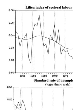
We claim that the explosion of unemployment in the 1990s is due to the erosion Ž of the conventional sources of industrial flexibility in Italy. If one compares Fig.
.
1 the pattern of intersectoral labour reallocation, as measured by the Lilien index, with the dynamics of unemployment from the 1950s through the 1990s, an interesting correspondence appears. In particular, it will be shown that there is a statistically significant negative correlation between unemployment and sectoral shifts of the labour force.
The relationship between unemployment and the dispersion of employment growth rates across different sectors and regions has been widely studied in the
Ž .
literature, following the path-breaking contribution of Lilien 1982 . We have tested the validity of the Lilien hypothesis for the Italian labour market and compared it with the US. The objective is to measure the relative importance of sectorial, regional and national factors in the explanation of the evolution of industry structure, and its impact on unemployment. We will show that sectoral dynamics and regional reallocations account for a great deal of the pattern of unemployment variation in Italy in the last decades. The ALilien hypothesisB
therefore appears to hold for Italy. However, the sign of the relationship is opposite to that predicted by Lilien and others, showing a different mechanism at play in Italy in relation to the US. In particular, sectoral and interregional reallocations in Italy reduce unemployment, rather than increasing it. This calls for a discussion of the policy and labour flexibility mechanisms underlying the operation of the labour market in Italy and Europe, as opposed to the US.
Ž .
Fig. 1. The relationship between sectoral labour reallocations and unemployment in Italy 1952–1994 .
The 1990s have marked the apex of a process of discontinuous but significant modernisation of the Italian labour market and society, in pursuit of the goal of greater European harmonisation. The AEuropeanisationB of the Italian labour market has entailed the abandonment of a few conventional sources ofA flexibil-ityB, such as the informal economy, the very small firms and recurrent
devalua-Ž
tions of the exchange rate see Garonna and Sica, 1997; Garonna and Gennari, .
1995 . It introduced more flexible policy and institutional mechanisms such as the deindexation of wages and temporary employment contracts. However, such changes have not fundamentally affected the two above-mentioned conditions prevailing in Europe of low cyclical responsiveness of industrial employment and high firing costs, while the traditional mechanisms permitting high levels of employment shifts among sectors and regions were gradually eroded. The increase in unemployment can be interpreted then as resulting from the various structural factors governing the intersectoral and interregional adjustments of the employ-ment structure in the process of greater European integration of the Italian economy and society.
The 1990s saw on one hand the end of the Italian specificity in Europe, but on the other hand, the emergence of the AEuropean deceaseB in Italy. Institutional reforms in fact did not eliminate rigidities characterising the Italian and European labour markets, in particular, those affecting the cyclical responsiveness of em-ployment, such as for instance the highly centralised wage bargaining structure or the lack of an effective safety net or welfare-to-work mechanism, and the regulation of hiring and firing. If Europe and Italy intend to maintain their
AmodelB of employment stability along the cycle and high firing costs, conditions will have to be created for greater intersectoral and interregional labour mobility. ByAAmericanisingB its employment shifting capacity, the European labour market can preventAAmericanisingBthe conditions of the employment contract. The case of Italy shows that if, and to the extent that, these conditions are not met, structural unemployment inevitably grows.
2. Sectoral shifts, aggregate shocks and the rise in unemployment
Linking employment trends in specific sectors with general macroeconomic conditions has traditionally been an area of policy discussion and controversy. Recently, attention has been focused on the relationship between intersectoral employment variations and aggregate unemployment dynamics. Sectoral patterns are, in fact, an essential component of labour market equilibrium and change. Labour market performance is crucially dependent upon the capacity of expanding
Ž . Ž .
Ž . leading to an increase in unemployment. Lilien in his seminal paper Lilien, 1982 claimed that as much as half of the cyclical variations in US unemployment were due to structural shifts in the sectorial composition of labour demand. On the other
Ž .
hand, high variability may: 1 facilitate adjustment to ever increasing changes in Ž .
technology and consumer preferences; 2 promote skill enrichment and employa-Ž .
bility; and, 3 induce cross-fertilization of experiences and institutional reform.
Ž . Ž . Ž .
Following Lucas and Prescott 1974 , Barro 1977 and Lilien 1982 , the economic literature has tested the relationship between unemployment and the dispersion of sectoral employment trends, the so-called Lilien index. Interesting
Ž .
theoretical developments have emerged: a aggregate demand shocks can also work through different sectors, therefore explaining, at least in part, the
relation-Ž
ship between unemployment and employment variability Abraham and Katz, . Ž .
1986 ; b sectoral variations can be anticipated on the basis of aggregate demand pressure or not anticipated when due to structural shifts at the sectorial level; therefore, the Lilien index can be decomposed into a predicted and a non-predicted
Ž . Ž .
element Neelin, 1987 ; and, c empirical analysis has in many cases confirmed the existence of a significant Lilien effect on unemployment, i.e. a positive relationship between unemployment and sectoral labour reallocations. It has, however, shown that endogenous industry shifts, i.e. shifts correlated with eco-nomic activity, also play an important part in explaining unemployment fluctua-tions. In short, the issue of whether sectoral shifts or aggregate shocks are explanatory factors, along with their relative importance and positive or negative impact on unemployment are empirical questions to be tested against available evidence.
In theory, the relationship between the variability of the industrial structure, as measured by the Lilien index st, and the rate of unemployment, depends on the
Ž .
following set of factors: 1 the extent to which sectors differ in their trend rates of Ž .
growth; 2 different sensitivity of various sectors vis-a-vis aggregate demand
`
Ž .
variations; and, 3 the degree of labour force homogeneity, mobility and labour market imperfection.
Ž .
It is worth noting that in the literature, conditions under 3 are conventionally
Ž . Ž .
labeled AstructuralB, and opposed to conditions under 1 and 2 , qualified as
Aaggregate demandB. In reality, structural and institutional factors are at play in all three sets of factors. Besides, both aggregate demand and structural factors evolve through time and may vary in different contexts. It is undeniable, however, that demand pressure cannot be considered unimportant in the working of the labour market and the evolution of industry composition of employment.
3. Industries’ growth rates and cyclical sensitivities
Ž .
Ž .
sufficient to produce a positive negative correlation between st and unemploy-ment.
Ž .
In the case of USA, Abraham and Katz 1986 showed that manufacturing employment grows less rapidly, but reacts more to the business cycle, while services grow more but with a minor cyclical sensitivity. We would then expect st
to move anti-cyclically in the US, and, indeed, many studies of North American Ž
labour markets have proved this to be the case see Abraham and Katz, 1986; .
Neelin, 1987 .
Even if differences in industry growth rates are unimportant, different sensitivi-ties in relation to the cycle generate a positive correlation between st and
Ž .
unemployment. Weiss 1984 showed that this is the case if hiring costs exceed firing costs, i.e. if firms find it easier to reduce employment rapidly than to increase employment rapidly, which is what takes place in the US. Even if aggregate demand were to remain stable, frictions and barriers in the labour market prevent an exact and instantaneous matching between employment losses in contracting firms and gains in expanding firms. Therefore, it is expected that higherst corresponds to higher unemployment rates.
Thus, predictions based on an analysis of all three sets of factors indicate for the US and North America, a positive correlation between st and the rate of
Ž
unemployment, which is what empirical analysis has consistently shown Abraham .
and Katz, 1986; Neelin, 1987 .
What can we say instead of the Italian labour market? Let us model it by considering a two-sector economy where sector 1 is services and sector 2 is manufacturing. Service employment is assumed to grow at a more rapid trend rate than manufacturing, and furthermore, to be more responsive to cyclical
move-Ž .
ments in gross national product GNP . We can formalize these assumptions by the following two-equation model:
ln E scqG tqg
Ž
lnYylnY).
Ž .
11 t 1 1 t t
ln E scqG tqg
Ž
lnYylnY).
2 t 2 2 t t
,where 1and 2 denote the service and manufacturing sector, respectively, and E1 and E are employment in the two sectors; Y is actual GNP and Y) is trend GNP
2 t t
obtained by applying the Hodrick–Prescott filter; G1 and G2 are the average growth rates of sectoral employment with G1)G2; g1 and g2 represent the
Ž responsiveness of sectoral employment to fluctuations in GNP withg1)g2 see
. Table 1, where DEVPIL express cyclical variations of output around its trend .
Using sectoral employment growth rates and sectoral shares in total employ-ment, we can construct a series of Lilien index, st, based on the dispersion in the rate of growth of employment across the two sectors:
1r2
E1 t 2 E2 t 2
sts
Ž
Dln E1 tyDln Et.
qŽ
Dln E2 tyDln Et.
.Ž .
2Table 1
a
Regressors Dependent variables
b c
lindt Lsvt
Ž .w x Ž .w x
Constant 8.5 526 0.00 8.3 738 0.00
d Ž .w x
Lt5180 0.13 22.5 0.00 –
Ž .w x
t5194 – 0.02 32.7 0.00
e Ž .w x
t8194 y0.02 y17.1 0.00 –
f Ž .w x Ž .w x
DEVPIL y0.14 y0.7 0.23 0.52 1.8 0.08
g Ž .w x Ž .w x
D8193 y0.05 y3.4 0.00 0.11 6.6 0.00
2
R 0.93 0.99
2
R 0.93 0.99
S.E. of regression 0.02, 177.4 0.03, 1078
w x w x
F-statistic 0.00 0.00
a Ž .
w x The t-statistic are in parentheses P; p-values in brackets P.
b
The logarithm of employment in industry.
c
The logarithm of employment in market services.
d
The logarithmic trend from 1951 to 1980.
e
The broken trend from 1981 to 1994.
f
The difference between the actual and the trend growth rate of GDP.
g
A step dummy from 1981 to 1993.
On the basis of the coefficients G1, G2,g1,g2 and of actual and trend rates of GNP growth, we can approximatest as follows:
)
sts 1r2
Ž
G1yG2.
q1r2Ž
g1yg2.
Ž
DlnYtyDlnYt.
.Ž .
3The values of the coefficients enable us to determine in theory howst moves over the business cycle:
s≠ ifDlnY)DlnY)
t t t
1 ifg yg )0 4
Ž .
1 2¦
sx ifDlnY )Ž .
-DlnY
t t t
sx ifDlnY)DlnY)
t t t
2 ifg yg -0
Ž .
1 2¦
s≠ ifDlnY )-DlnY
t t t
.
Thus, if service employment is, as we assumed, more responsive to cyclical movements in GNP than manufacturing, the second term in the approximate
Ž .
formula forst is positive negative when the actual rate of GNP growth exceeds Žfalls short of the trend rate of GNP growth, so that the value of. st increases during upturns and decreases during downturns in the economy.
but a step dummy was introduced from 1981 onwards to account for a shift in the pattern, which corresponds to theAspongeB function played by services in relation
Ž .
to the industrial employment shake-out Garonna, 1994 .
The model specification is based on our understanding of the patterns of employment growth in Italy in the different sectors and on empirical evidence reflecting these patterns. In particular, industrial employment followed two distinct and different patterns, in relation to the two phases of industrialisation in the 1950s, 1960s and 1970s, and deindustrialisation in the following period. There-fore, in order to reproduce econometrically the industrial employment series, we regressed the actual series on a broken trend. Precisely, we fit an increasing
Ž .
logarithmic trend from 1951 to 1980 lt5180 because in this period, the growth rate of employment is exponential corresponding to the phase of sustained
Ž .
industrialisation in Italy, and a decreasing linear trend from 1981 to 1994 t8194 justified by the fact that throughout this period, industrial employment decreased at a constant rate corresponding to the deindustrialisation phase. Finally, a step dummy was included for the period 1981–1993 to account for the downward shift of the employment level, corresponding to the process of employment expulsion from manufacturing towards the tertiary. The existence of a broken trend is confirmed by the estimated coefficient’s sign, positive for lt5180 and negative for t8194; as expected, the step dummy has a negative coefficient.
To describe the employment series in the service sector, we introduced a linear trend for the whole period. Actual series are in fact always increasing in the whole period. The process of terziarization of the Italian economy has proceeded following a continuous pattern in the post-war period. Growth in service employ-ment, however, was affected by the industrial shake-out in the 1980s; the inclusion of a step dummy for the period 1981–1993 is justified by theAspongeB function which services had to play in relation to the release of surplus labour from the large industrial firms. As expected, the dummy has a positive sign.
In both regressions, we introduced also a cyclical indicator, represented by DEVPIL, i.e. the difference between the actual and the trend growth rate of GDP. The year 1980 represents a crucial year for understanding the patterns of employment growth in Italy. Three main institutional factors account for this year
Ž .
marking the shift from industrialisation to deindustrialisation: 1 In 1980, there
Ž .
was a strike of middlemanagers in Turin cadre , the so-called Amarch of the 40,000B, which marked the defeat of the labour unions, and the passage to a different phase of industrial relations, characterised by softer and less antagonistic Ž . aptitudes, and therefore, the end of the resistance to lay-offs and dismissals. 2 Legislation and practices concerning Cassa Integrazione Guadagni, a subsidy scheme for lay-offs and short-time working, were enhanced. This made it possible
Ž .
to shake out labour from large industrial firms. 3 There was a change in monetary policy due to the political decision to link the exchange rate at the
Ž .
binding for enterprises, namely large industrial firms. While they were used to recurrent exchange rate adjustment in the past and accommodating monetary policy, they knew that these patterns could not go on, and they had to put their house in order.
The post-1980 dummy and the break in the trends in this year are justified by these institutional factors, which correspond to a change in the labour market climate and in the employment model.
We checked the sensitivity of the main results to alternative assumptions. In particular, we tested the following alternative specifications of the model:
Ž
1. regression of the cyclical component of the employment series original series .
minus the trend component obtained from the Hodrick–Prescott filter for both industry and services on a constant and DEVPIL;
2. regression of the employment series in logarithmic terms on a constant and the trend component obtained by the Hodrick–Prescott filter and DEVPIL.
Both specifications gave about the same absolute value and the same sign for
Ž .
the coefficient of the cyclical elasticity of employment DEVPIL as the adopted model. This shows that the current specification can be considered sufficiently robust.
The estimated coefficients of the trends are highly significant at any signifi-cance level and show the expected sign. The coefficient of cyclical sensitivity of industry is negative, but not significant. The estimated one for services is positive
Ž . Ž
and significant at the 10% significance level , as are all other coefficients see .
Table 1 .
The empirical test of the model then confirms that in Italy, the responsiveness of services employment to GDP fluctuations is higher than that of industrial employment, and thereforeg1yg2 is positive. This is a major difference charac-terizing the Italian and European labour markets vs. the North American ones, and accounting for an expected negative correlation between st and unemployment.
Ž .
The breakdown of the series see Table 2 shows that the sectors having greater cyclical sensitivity are those characterized by small firms or by greater exposure to international competition. This is the case with means of transport, mechanical equipment, chemicals, metals, rubber, etc. In the other sectors, employment protection legislation, sheltered product market conditions, subsidized lay-off programmes and other institutional arrangements reduce the cyclical responsive-ness of employment variations. This is the case, for instance, with the highly regulated distributive trade sector, but is also true ofAother manufacturingB.
Table 2
The elasticity of employment growth with respect to cyclical GDP fluctuations
Branches Elasticities t-Statistic
Energy 0.21 2.1
Ferrous and non-ferrous metals 0.37 1.6
Non-metalllic minerals 0.44 1.9
Chemical and pharmaceutical 0.58 2.6
Mechanical industry 0.89 4.9
Means of transport 0.95 4.6
Food, drink and tobacco 0.13 1.0
Textile and clothing 0.33 1.9
Timber and wooden furniture 0.27 1.6
Paper and printing 0.49 2.9
Rubber and plastic 0.66 2.8
Other manufacturing 1.06=10ey6 2.0
Wholesale and retail distribution 1.5=10ey7 0.6
Hotels and catering 0.21 1.2
Transport and communications 0.21 8.1
Ž
Elasticities are calculated regressing the rate of growth of employment in each branch logarithmic
.
prime differences on the current and lagged values of the difference between the actual and trend GDP growth rates, plus the trend and a constant, using OLS with annual data for the sample 1951–1994.
This picture contrasts with the one presented in the analysis of US labour
Ž .
market Abraham and Katz, 1986 where the job creating sectors were the more stable ones, and therefore, variability appeared to create turbulence and friction, thereby feeding unemployment.
This contrast is also apparent in relation to hiring and hiring costs. Contrary to
Ž .
what Weiss 1984 showed for the US, firing costs in Italy tend to be higher than hiring costs. In a heavily regulated labour market such as Italy’s, constraints on firing are much bigger than on hiring; considering the slack in the market, the existence of training provisions and institutions, the role played by small firms, job search assistance, and the management philosophy prevailing among European business, hiring arrangements have proved to be much less costly. A recent study ŽJaramillo et al., 1992 showed that labour adjustment costs in Italy have been. significantly asymmetric: particularly for large firms, the costs of separations appear dominant vis-a-vis those of accessions. This is explained by reference to
`
of employment and structural dynamics. When and if this dynamics is stifled and eroded, as it was the case for Italy, unemployment would tend to grow.
However, theory would also predict that the degree of labour market imperfec-tion and other fricimperfec-tions associated with labour intersectoral shifting be positively correlated with unemployment, as in Lilien.
It is necessary, therefore, to verify against empirical evidence how the different factors affect the relationship between st and unemployment, and which factors play a relatively greater importance.
4. Anticipated and unanticipated variability
Ž .
Following Neelin 1987 , we developed a model for testing the relationship between unemployment and employment variability in the Italian labour market using annual data from 1951 to 1994.
We intend to test whether shifts in the composition of labour demand have caused fluctuations in the aggregate unemployment rate.
The model must capture the fact that, as we discussed, different sets of explanatory factors lead to contrasting predictions in the relationship: in particular, we have seen that there are structural aggregate demand factors affecting
posi-Ž .
tively the relationship between variability and employment anti-Lilien , and
Ž .
frictional factors exerting a negative influence pro-Lilien .
We need to construct then the independent variable, st, distinguishing between
Ž .
the endogenous shifts working through aggregate demand factors and the
exoge-Ž . Ž .
nous frictional shifts . This was done, following Barro 1977 , Abraham and Katz Ž1986 , and Neelin 1987 , by introducing two distinct measures of sectoral labour. Ž . reallocations: the predicted Lilien index, measuring the anticipated shifts induced by structural and labour demand factors, and the unpredicted Lilien index, capturing frictional unanticipated variations. We proceed in three stages.
Ž .1 First of all, we construct an aggregate demand indicator. The unanticipated money growth rate can be taken as a proxy of swings in aggregate demand. This variable is constructed as the difference between the actual money growth rate series and the estimated one from the regression of the actual money growth rate on a constant, the two periods lagged values of the money growth rate, the difference between the actual public expenditure and the forecasted one, the ratio of unemployment rate to employment rate.
Ž .2 Second, we determine the predicted values of sectoral and total rates of growth of employment. They were calculated by regressing the employment growth rates on a constant, the current and one lagged values of unanticipated money growth rate and a time trend:
˙
˙
where li tslog ltyloglty1 is the employment growth rate of i, where i indicates the following sectors.
Similarly, we estimate the aggregate employment growth rate:
˙
Ltscqa resM21 tqa resM22 ty1qa TREND.3
Together with the current value of the growth rate of unanticipated money supply, one lagged value has been included in the regressions since sectoral and aggregate employment growth rates do not necessarily adjust instantaneously to aggregate shocks. The trend variable captures the demographic and other changes which may have occurred in the labour market over the period.
However, the unanticipated money growth rate may not account for all the aggregate effects on both the sectoral and the aggregate employment growth rates. In order to capture the aggregate residual effects, we construct a variable using the weighted average of the residuals from the above regressions where the weights are the employment shares of each sector in the total employment. This variable has been included as an independent variable, together with the current and lagged money growth rate and the trend variable, in a further set of employment growth rate equations:
˙
li tscqa resM21 tqa resM22 ty1qa TREND3 qa mpe14 i t
˙
Ltscqa resM21 tqa resM22 ty1qa TREND3 qa mpe1 ,4 t
where mpe1tse1 li t i trÝi i tl is the weighted averages of the residuals from the estimated regressions for each sector where the employment shares of each sector in the total employment li trÝi i tl are utilized as weights.
By subtracting from the actual employment growth rates, sectoral and total the estimated residuals, we obtain the corresponding fitted employment growth rates series, sectoral and total, respectively:
ˆ
˙
˙
li tye2i tsli t is the estimated employment growth rate for each sector;
ˆ
˙
˙
LtyE2i tsL is the estimated total employment growth rate.t
Ž .3 Third, on the basis of the fitted series at sectoral and aggregate level, we calculate the predicted part of the Lilien index using the weighted average of the squared deviations between the sectoral fitted employment growth rates and the total one, where the weights are the actual employment shares in total employ-ment:
1r2
23 2
ˆ
ˆ
˙
˙
stŽp.s
Ý
li trL ltž
i tyLt/
.Ž .
61
new residuals series by subtracting the fitted series from the actual one. On the basis of the residuals series, sectoral and total, we calculate theAunpredictedB part of Lilien index:
1r2 23
2
stŽnp.s
Ý
li trL e3tŽ
i tyE3t.
.Ž .
71
[image:13.595.47.387.192.457.2]This index captures the impact of sectoral specific shocks on the employment sectoral shifts.
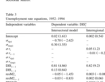
Table 3
Unemployment rate equations, 1952–1994
a
Independent variables Dependent variable: DISt
Intersectoral model Interregional models
Ž . Ž . Ž .
Intercept 0.02 1.61 0.002 0.54 0.02 0.54
Ž .
stŽp. y0.70 y2.62 – –
Ž .
stŽnp. 0.30 1.55 – –
Ž .
srt – 0.05 1.2 –
Ž .
srty1 – y0.01 y0.27 –
Ž .
srtŽp. – – y0.28 y2.6
Ž .
srtŽnp. – – 0.16 2.1
Ž . Ž . Ž .
DISty1 0.81 4.86 0.82 9.2 1.14 7.1
Ž . Ž .
DISty2 0.13 0.84 – y0.01 y1.14
Ž . Ž . Ž .
resM2t y0.05 y1.45 0.003 y0.08 0.003 0.08
Ž . Ž . Ž .
resM2ty1 y0.03 y0.83 0.002 0.06 0.02 0.51
Ž .
TREND – 0.0005 1.8 –
2
R 0.93 0.93 0.92
2
R 0.91 0.91 0.91
S.E. of regression 0.007 0.007 0.007
w x w x w x
F-statistic 67.2 0.00 66.2 0.00 63.2 0.00
w x w x w x
Ljung–Box Q-statistic 14.4 0.81 7.29 0.99 23.3 0.18
w x w x w x
Durbin’s h y1.02 0.31 0.03 0.98 0.72 0.47
w x w x w x
Augmented Dickey–Fuller y7.9 0.00 y5.5 0.00 y6.5 0.00
w x w x w x
ARCH test 0.16 0.97 0.79 0.37 0.75 0.39
w x w x w x
Chow test 0.82 0.56 0.26 0.96 2.4 0.05
w x w x w x
Jarque–Bera normality test 0.42 0.81 1.3 0.51 2.3 0.31
w x w x w x
CUSUM test 0.91 0.06 0.64 0.33 1.1 0.02
The models are estimated using OLS with annual data for the sample period 1952–1994 in the aggregate version and 1952–1993 in the regional version. The dependent variable DISt is the unemployment rate series which has a mean of 0.08 and a standard deviation of 0.02;st is the total Lilien index which at aggregate level has a mean of 0.03 and a standard deviation of 0.01;stŽp. and stŽnp. are the Lilien predicted and unpredicted index, respectively; sr is the regional Lilien indext
which has a mean of 0.03 and a standard deviation of 0.04;srtŽp.and srtŽnp. are the predicted and unpredicted part of the regional Lilien index, respectively.
Quite similar results are obtained by taking as a dependent variable the unemployment rate in its strict sense as opposed to that which include those who are seeking employment.
a Ž . w x
We can now proceed to test the model including both the predicted and unpredicted Lilien indices among the independent variables to explain the
unem-Ž .
ployment rate see Table 3 . The other independent variables are the lagged unemployment growth rate itself, and both the current and the lagged values of the unanticipated money growth rate.
The results are statistically significant and confirm our ex ante hypothesis. The coefficient of theApredictedB index is negative and significant at the 5% significance level, meaning that sectoral shifts which can be attributed to aggregate economic activity cause changes in the unemployment rate in the opposite direction. In particular, a rise in the ApredictedB Lilien index, corresponding to
Ž .
increases in the positive andror negative deviations between the sectoral em-ployment growth and the total one caused by aggregate demand, produces a decrease in the aggregate unemployment rate. The coefficient of the Lilien
AunpredictedB index is positive and significant at the 10% significance level; therefore, also frictional sector-specific shocks influence the Italian aggregate unemployment rate. In particular, a rise in the unpredicted index, which
corre-Ž .
sponds to increases in the deviations positive andror negative between the sectoral employment growth rates and the total one caused by exogenous shift, increases aggregate unemployment. The lagged value of the aggregate unemploy-ment rate itself is positive and highly significant denoting a strong persistence in the unemployment rate series, while the two period lagged value is not signifi-cantly different from zero. On the basis of Adjusted R-squared, the standard error of regression, the F-statistic and the Q-statistic, the estimated regression repre-sents a good fit.
In conclusion, the empirical test confirms that high intersectoral employment variability in Italy has been associated with low unemployment; in the 1970s and throughout the 1980s, but above all in the 1990s, variability diminished and unemployment rose correspondingly. Employment restructuring and sectorial re-conversion in Italy was sustained essentially by demand pressure and employment creation. New jobs pulled human resources from declining sectors, assuring fluidity to labour market mechanism.
5. The impact of regional employment shifts
Interregional shifts closely interact with intersectoral ones. Localization factors have played an important role in Italian economic development, where new
Ž .
expanding areas have attracted business and jobs in the so-called Adriatic belt and declining ones have faced reconversion and labour shedding. In order to take into account the territorial dimension of employment variability, we constructed a regional Lilien index, measuring regional shifts in employment, and analysed it in the framework of the set of relationships between variability and unemployment
Ž .
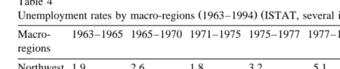
Table 4
Ž . Ž .
Unemployment rates by macro-regions 1963–1994 ISTAT, several issues-a
Macro- 1963–1965 1965–1970 1971–1975 1975–1977 1977–1983 1983–1991 1991–1995 regions
Northwest 1.9 2.6 1.8 3.2 5.1 6.4 6.7
Northeast 3.0 3.0 2.4 3.1 5.1 6.0 6.2
Centre 3.0 3.7 3.5 5.0 5.7 8.3 9.0
South 3.7 4.5 5.0 6.8 10.7 17.4 17.8
The regional shift index is calculated taking the square root of the weighted sum of the variances of regional employment growth rates using as weights the employment share of each region on the total employment:
1r2
19 2
˙
˙
sts
Ý
ljtrLt=ž
ljtyLt/
,Ž .
8js1
Ž
where ljtrL is the employment share of the region jt s1, . . . , 19 Molise was joint with Abruzzi until 1965, so we have 19 rather than 20 NUTS-II regions in
˙
˙
.
Italy ; l and L are the employment growth rates, regional and total, respectivelyjt t
˙
in terms of logarithmic first differences ljtslog ltylog lty1.
Following the model described above, we regress the unemployment rate on a constant, one lagged value of the unemployment rate itself, the current and lagged values of the regional shifts index, the current and lagged value of the unantici-pated money growth, and a time trend.
Table 3 summarizes the results of the estimates, confirming a priori hypotheses and closely corresponding to those obtained considering intersectoral variations. The coefficient of the predicted regional Lilien index is negative and significant; the non-predicted regional index is on the contrary positive and significant; therefore, both frictional unemployment-creating effects and structural labour demand employment-creating effects were at play in accounting for interregional mobility. In other words, the regional reallocation of labour has created some unemployment due to frictions and barriers to mobility, but this effect has been more than compensated for by the employment creation effect of labour realloca-tion which, by shifting labour away from declining regions to areas of economic expansion, kept unemployment under control. In the later part of the period, interregional employment reallocation declined, the market became ossified at the regional level, and unemployment climbed steeply.
It is worth noting that the sectorial Lilien effect is six times greater than the
Ž .
direction. Moreover, the lagged value of the unemployment rate is highly signifi-cant denoting a strong persistence in unemployment.
6. Conclusions: the erosion of conventional sources of labour flexibility
We can conclude on the basis of empirical evidence that what contributed to stifling and drying out the intersectoral and interregional flows of employment restructuring also contributed to the increase in unemployment in Italy. The econometric exercise points out that the relationship between employment variabil-ity and unemployment is robust and empirically founded. The model illustrates a pattern of labour market flexibility which characterizes the Italian case, but also the broader European one, as compared to better known North American or Asian models. New hires, employment creation, sectoral restructuring and regional mobility, which has kept unemployment down, rather than employment stability, intrafirm careers and the consolidation of already strong and successful sectors or enterprises. Or better, it is the lack of labour reallocation and sectoral shifts, their exhaustion in the passage from 1950s–1960s to 1970s and 1990s, which is at the root of the Italian and European employment sclerosis.
Variability and employment reallocation in the framework developed here reflect and call into question the operation of the structural and demand factors affecting labour mobility and flexibility. These factors are deeply rooted in the institutions and nature of Italian society: for instance, the role of the family in bearing the costs of unemployment and in the informal economy, or theApolitical exchangeB with unions, or the dynamism of small and medium size enterprises. These factors created the conditions for the progressive adjustment of the labour market to successive waves of structural change through intersectoral and interre-gional employment shifts. At each wave, however, the responsiveness of the labour market weakened and lagged behind; correspondingly, the rate of unem-ployment has been steadily rising. The widening tax and social security wedge has hit particularly strongly small firms; the informal economy has been severely constrained by fiscal consolidation filling the loopholes of tax evasion and erosion; income transfers towards the aged and less mobile segments of a rapidly aging population have had disincentive effects to relocation of business and labour. These developments in the context of rigid hiring and firing mechanisms and narrow wage differentials, highly regulated product and housing markets and weak infrastructures, explain how and why the flexibility patterns of the Italian labour market were lost in the 1990s.
increasingly competitive environment; what is the most appropriate policy mix between labour mobility and flexibility.
7. Data sources
Aggregate data on sectoral employment from 1970 to 1994 are the official
Ž .
ones, as provided by the National Statistics Institute ISTAT . For the period Ž
1951–1969, the series are drawn from a data bank see Golinelli and Mon-.
terastelli, 1990 reconstructed on the basis of national accounts estimates. At the regional level, employment data are the official ones for the period 1980–1993. From 1951 to 1959, the series have been reconstructed on the basis of unpublished ISTAT data; from 1960 to 1979, the series are drawn from the volume AOccupati per Attivita economica e Regione
`
B in ISTAT ACollana diŽ .
informazioniB, 1981 and 1982, no. 3 and no. 4 ISTAT, several issues-b . The sectors considered are the following: agriculture; energy; ferrous and non-ferrous metals; non-metallic mineral products; chemical products; mechanical industry; means of transport; food, drink and tobacco; textile and clothing; timber, wooden products and furniture; paper and printing products; rubber and plastic products; other manufacturing industries; building and construction; total manufacturing industry; wholesale and retail trade; lodging and catering services; transport and communication services; services of credit and insurance institutions; business services provided to enterprises; public administration; other non-marketed ser-vices. It would have been interesting to replicate the test in Abraham and Katz Ž1986 by using in the unemployment regressions the number of vacancies as the. dependent variable. However, unfortunately, vacancy data are not available for Italy.
Ž .
The money series M2 for the period 1975–1994 is provided by the Bank of
Ž .
Italy Banca d’Italia, various years , while from 1951 to 1974, the data bank of
Ž .
Fratianni–Spinelli Fratianni and Spinelli, 1991 is used .
The unemployment series is drawn from ISTATAAnnuario Statistico ItalianoB
Ž .
for the period 1952–1994 ISTAT, several issues-a and from ISTATARilevazioni Ž
Campionarie delle Forze di LavoroB for the period 1959-1994 ISTAT, several .
issues-c .
Acknowledgements
This paper was drawn from a larger work on AFlexibility Mechanism in Post-War ItalyB produced in the framework of the Kiel Institute Project on the
Social Market Economy. We acknowledge useful comments and help from R.
References
Abraham, K.G., Katz, L.F., 1986. Cyclical unemployment: sectoral shifts or aggregate disturbances.
Ž .
Journal of Political Economy 94 3 , 507–522.
Ž .
Banca d’Italia. Bollettino Statistico, 1975–1994, Rome various years .
Barro, R.J., 1977. Unanticipated money growth and unemployment in the United States. American
Ž .
Economic Review 67 2 , 101–115.
Fratianni, M., Spinelli, F., 1991. Storia monetaria d’Italia: l’evoluzione del sistema monetario e bancario. Arnoldo Mondadori, Milan.
Garonna, P., 1994. La parabola dei servizi in Italia: dal decentramento produttivo alla
deterziariz-Ž .
zazione. In: Pizzuti, F.R. Ed. , L’economia Italiana Dagli Anni Settanta Agli Anni Novanta. McGraw-Hill, Rome, pp. 395–418.
Garonna, P., Gennari, P., 1995. Il ruolo economico delle relazioni industriali. Lavoro e Relazioni Industriali 1, 5–38.
Garonna, P., Sica, F., 1997. Intersectoral labour reallocations and flexibility mechanisms in post-war
Ž .
Italy. In: Siebert, H. Ed. , Sectoral Structural Change and Labour Market Flexibility: Experience in Selected OECD Economies. Mohr Siebeck, Tubingen.¨
Golinelli, R., Monterastelli, M., 1990. Un metodo per la ricostruzione di serie storiche compatibili con la nuova contabilita nazionale. Prometeia, Nota di lavoro 451, Bologna.`
Ž .
ISTAT. Annuario Statistico Italiano, 1951–1994, Rome several issues .
ISTAT. Occupati per attivita economica e regione. Collana di informazioni, 1981 no. 3 and 1982 no. 4,`
Ž .
Rome several issues .
Ž .
ISTAT. Rilevazioni Campionarie delle Forze di Lavoro, 1959–1994. Rome several issues . Jaramillo, F., Schiantarelli, F., Sembenelli, A., 1992. Costi di aggiustamento asimmetrici nei modelli di
domanda di lavoro: una verifica empirica su dati disaggregati. Ricerche Applicate e Modelli per la Politica Economica II, Banca d’Italia.
Ž .
Lilien, D.M., 1982. Sectoral shifts and cyclical unemployment. Journal of Political Economy 90 4 , 777–793.
Lucas, R. Jr., Prescott, E.C., 1974. Equilibrium search and unemployment. Journal of Economic
Ž .
Theory 7 2 , 188–209.
Neelin, J., 1987. Sectoral shifts and Canadian unemployment. The Review of Economics and Statistics
Ž .
69 4 , 718–723.