www.elsevier.nlrlocatereconbase
Replication study
Reapplication and extension: intergenerational
mobility in the United States
Alison Aughinbaugh
)Bureau of Labor Statistics, Room 4945, Postal Square Building, 2 Massachusetts AÕe. NE, Washington, DC 20212, USA
Received 1 February 2000; accepted 7 September 2000
Abstract
w Ž . x
This paper replicates and extends Solon’s Am. Econ. Rev. 82 1992 393–408. article
AIntergenerational Income Mobility in the United States B. The results confirm previous findings about the degree of transmission in earnings and consumption from fathers to sons. The correlation between fathers’ and sons’ earnings lies in the neighborhood of 0.4 and the correlation in consumption is larger. Using the sons’ outcomes when they are 5 years older does not alter the estimates of the correlation in earnings, but the estimates of the correlation in consumption are smaller and closer to the estimates of the correlation in earnings. The estimates that use consumption data are sensitive to whether sons’ 1984 or 1989 outcomes are used and to whether one adjusts for family size and structure.q2000
Elsevier Science B.V. All rights reserved.
JEL classification: J1
Keywords: Transmission; Status; Intergenerational; Father; Son
1. Introduction
Ž .
In the June 1992 issue of the American Economic ReÕiew, Solon 1992 presents new estimates of the intergenerational correlation in income for the US.
Ž .
The estimates he reports, as well as those Zimmerman 1992 reports in the same issue of the ReÕiew, are in the neighborhood of 0.4. Their work points toward less
)Tel.:q1-202-691-7520; fax:q1-202-691-7425.
Ž .
E-mail address: aughinbaugh [email protected] A. Aughinbaugh .–
0927-5371r00r$ - see front matterq2000 Elsevier Science B.V. All rights reserved.
Ž .
mobility in status across generations than was suggested by earlier work.1 Recent studies have found both greater and less mobility than that estimated by Solon or Zimmerman.2After attempting to replicate Solon’s results for earnings, I consider how the relative youthfulness of the sons in Solon’s sample affects the results by estimating the intergenerational correlations later in the sons’ lives and by looking at different measures of status for fathers and sons.
First, I compare the estimates when earnings are used to proxy for status, and sons’ earnings from 5 years later are used in the estimation. Second, I examine the effects of using data on consumption as opposed to earnings to measure economic status.
Using data on sons from 5 years later produces estimates of the correlation in earnings that are about 0.4. In contrast, the results using consumption data point to greater transmission of status than do those using earnings data. The consumption results that use later data are smaller and more similar to the results that use earnings than the consumption results that use the earlier data, particularly when family size is accounted for. As a whole, the results indicate that consumption is transmitted to children to a greater extent than are earnings. This is feasible if saving behavior is transmitted or if transfers which make the consumption patterns of the two generations more similar are passed between parents and children.
2. Results using earnings
I draw two samples from the PSID using Solon’s selection criteria. Sons in the samples were born between 1951 and 1959, have positive earnings in 1984, and are from original PSID families that were headed by men. Sons from the original
Ž .
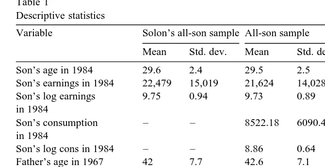
Survey of Economic Opportunity SEO component of the PSID, which over-sam-ples low-income households, are omitted. The sample of all father–son pairs that meet these criteria has 428 observations while Solon’s sample contained 433. Of the pairs in the all-son sample, the eldest sons are retained in the eldest-son sample. My eldest-son sample contains 322 pairs while there were 330 father–son pairs in Solon’s. Although I have not succeeded in extracting Solon’s exact samples, the samples used in this study are quite similar to his. Table 1 reports descriptive statistics for Solon’s all-son sample and my all-son and eldest son samples. The descriptive statistics for the two all-son samples are nearly identical. As in Solon’s work, all monetary variables are transformed into 1984 dollars.
Solon points out that averaging the father’s log earnings reduces the measure-ment error associated with using a snapshot of father’s earnings to proxy for
1 Ž .
See Becker and Tomes 1986 for an extensive review of earlier work.
2 Ž . Ž .
Mulligan 1997 and Lillard and Kilburn 1997 are examples of recent work that estimate less
Ž . Ž .
Table 1
Descriptive statistics
Variable Solon’s all-son sample All-son sample Eldest-son sample Mean Std. dev. Mean Std. dev. Mean Std. dev.
Son’s age in 1984 29.6 2.4 29.5 2.5 29.6 2.5
Son’s earnings in 1984 22,479 15,019 21,624 14,028 21,860 12,996
Son’s log earnings 9.75 0.94 9.73 0.89 9.75 0.89
in 1984
Son’s consumption – – 8522.18 6090.48 8608.99 6291.09
in 1984
Son’s log cons in 1984 – – 8.86 0.64 8.86 0.66
Father’s age in 1967 42 7.7 42.6 7.1 42.7 7.4
Father’s earnings in 1967 29,304 20,015 29,429 20,926 29,342 20,787
Father’s log earn in 1967 10.1 0.69 10.1 0.68 10.09 0.7
Father’s consumption – – 6524.32 2909.65 6675.57 3005.97
in 1967
Father’s log cons in 1967 – – 8.69 0.46 8.71 0.46
Number of observations 433 428 322
permanent earnings, and thus reduces the downward bias of OLS estimates. Consequently, he uses father’s earnings from 1967 to 1971 and multi-year averages of earnings to proxy for father’s status to estimate the degree of intergenerational mobility.
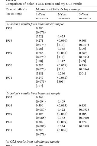
Table 2 compares Solon’s results from this procedure with my results. Panels a and b of Table 2 present Solon’s results from the unbalanced and balanced samples.3 Panels c and d present the analogous results from the samples used in this paper. The differences between the two sets of results are small, and I believe that they arise from differences in the samples.
Ž .
Instrumental variables IV can also be used to reduce the error-in-variables problem associated with the measurement of father’s status. In Solon’s use of this technique, the number of years of schooling that the father has completed by 1968 serves as an instrument for father’s status. The PSID’s 1968 information on education is in interval form. Solon assigns the father’s years of schooling to be the midpoint of the reported interval except for fathers in the highest category, who are assigned 18 years of schooling. My IV estimate of the correlation between
Ž .
the two generations’ outcomes is 0.552 SEs0.132 while Solon’s IV estimate is
Ž .
0.526 SEs0.135 . Solon points out that father’s education may not be a valid
3
Table 2
Comparison of Solon’s OLS results and my OLS results Year of father’s Measures of father’s log earnings
log earnings 1-Year 2-Year 3-Year 4-Year 5-Year
measures measures measures measures measures
( )a Solon’s results from unbalanced sample
1967 0.386
1969 0.285 0.081 0.369 0.088 0.413
Ž0.073. w317x Ž0.083. w301x Ž0.093.
( )b Solon’s results from balanced sample
1967 0.369
1969 0.406 0.088 0.405 0.094 0.413
Ž0.085. 0.382 Ž0.090. 0.397 Ž0.093. ( )c OLS results from unbalanced sample
1967 0.398
1969 0.282 0.085 0.506 0.098 0.447
Ž .
Table 2 continued
Year of father’s Measures of father’s log earnings
log earnings 1-Year 2-Year 3-Year 4-Year 5-Year
measures measures measures measures measures
( )d Solon’s results from unbalanced sample
1967 0.389
1969 0.274 0.083 0.431 0.095 0.447
Ž0.070. 0.413 Ž0.090. 0.420 Ž0.098.
Standard errors are in parentheses. Sample sizes are in brackets for the unbalanced samples, and are 290 and 280 for Solon’s and my balanced samples, respectively.
instrument but may belong in the model for son’s status as a regressor. If that is
Ž
the case and if father’s education is positively related to his son’s earnings as is
.
likely , the IV estimates will be upwardly inconsistent.
My estimates present the same picture as those in the work of Solon. Both sets of estimates imply that the correlation between son’s and father’s earnings lies in the neighborhood of 0.4.
If the earnings of the sons do not reflect their socioeconomic status because of their youth, then examining them at older ages may provide more accurate estimates of intergenerational income mobility. I explore this possibility by using
Ž . 4
sons’ outcomes 5 years later in 1989 to measure status.
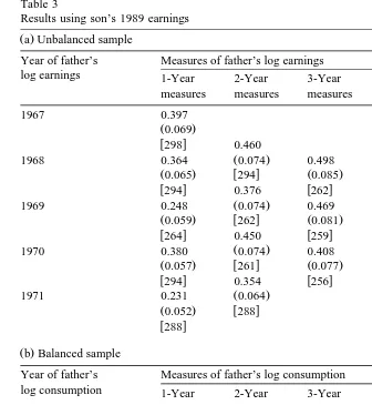
Table 3 reports the results using the 1989 son outcomes. When 1989 earnings data are used for the sons and a 5-year average of earnings for the fathers, the
Ž .
estimate of the intergenerational coefficient is 0.466 SEs0.087 . Using the 1984
Ž .
earnings data produced an estimate of 0.447 SEs0.098 . The correlation esti-mates using the 1989 earnings are similar, but slightly greater than the correlations in father’s and son’s earnings using 1984 measures for sons.5 When father’s
4
Between 1985 and 1990, 32 sons were lost from the sample because of attrition. Thus, the sample used here is not identical to that used to produce the estimates in Table 2. The sons who attrited tend to be those who had low 1984 earnings andror whose fathers reported low earnings in 1968–1972. For comparison, Appendix A presents the estimates using 1984 earnings and the sample still in the survey
Ž .
in 1990. Similar to the results in Fitzgerald et al. 1998 , the estimates of the intergenerational coefficient are slightly higher for the non-attriting sample, but the differences are not different from zero. As Fitzgerald et al. point out, some attrition will have occurred prior to 1984 and thus the estimates may already be biased.
5 Ž .
Table 3
Results using son’s 1989 earnings
Ž .a Unbalanced sample
Year of father’s Measures of father’s log earnings
log earnings 1-Year 2-Year 3-Year 4-Year 5-Year
measures measures measures measures measures
1969 0.248 0.074 0.469 0.086 0.466
Ž0.059. w262x Ž0.081. w259x Ž0.087.
Year of father’s Measures of father’s log consumption
log consumption 1-Year 2-Year 3-Year 4-Year 5-Year
measures measures measures measures measures
1969 0.228 0.073 0.426 0.086 0.466
Ž0.062. 0.398 Ž0.081. 0.430 Ž0.087.
Standard errors are in parentheses. Sample sizes are in brackets for the unbalanced sample. The sample size for the balanced sample is 254.
earnings are instrumented for, the estimate of the intergenerational coefficient is
Ž .
3. Results using consumption data
Consumption can be argued to be superior to earnings as a proxy for permanent status.6 In this sample, consumption will be a better measure of status than earnings if sons who will eventually have high earnings receive intergenerational transfers that augment their earnings or are able to borrow against their future
Ž .
earnings in their early years i.e., via mortgages . Children whose parents have higher incomes and more wealth are more likely to receive transfers and these transfers are compensatory, that is, the less well-off children in a family receive
Ž .
them Altonji et al., 1992; McGarry, 1997; McGarry and Schoeni, 1996, 1997 . The PSID does not contain a complete measure of household or individual consumption, but does provide data on family spending on food eaten at home, food eaten out, rent, and the value of owned housing. These components of consumption are used to construct several proxies of status. The proxies are the sum of food expenditures, weighted sums of the available components of con-sumption, and a predicted value of earnings.7 I treat family size and structure in
Ž . Ž .
three ways: 1 no adjustment is made, 2 the proxies are divided by household
Ž .
size, and 3 the proxies are divided by adult equivalents using a scale where each adult equals 1 and each child equals 0.4.8
Ž .
The weights for the weighted sums are from Skinner 1987 . Skinner estimates the weights by regressing total consumption on the four categories of spending
Ž .
using data from the Consumer Expenditure Survey CEX . He estimates two sets of weights, one from the 1972–1973 CEX and one from the 1983 CEX. I use three combinations of the weights to estimate the degree of intergenerational mobility:
Ž .1 the 1972–1973 weights are used to construct the proxies for fathers and sons
wFS7273 , 2 the 1983 weights are used to build the proxies for fathers and sonsx Ž . wFS83 , and 3 the 1972–1973 weights are used to build the fathers’ proxy and thex Ž .
w x
1983 weights are used to build the sons’ proxy F7273S83 .
Additionally, a predicted value of permanent status is constructed using the available data on consumption. To construct the predicted value, earnings are regressed on the four components of consumption.9 The predicted values contain
Ž .
the permanent portion of earnings. Dearden et al. 1997 show that when predicted values are used to estimate the intergenerational coefficient, the results may either over- or under-estimate the true value depending on whether the unobserved
6 Ž .
For instance, Attanasio and Browning 1995 find that after controlling for family composition, the age profile for consumption isAremarkably flat.B
7 Ž .
The sum of food expenditures is used as a proxy for consumption in Altonji et al. 1992 . The
Ž . Ž .
weighted sum is used to proxy for consumption by Becker and Mulligan 1997 and Mulligan 1997 .
Ž .
Dearden et al. 1997 use predicted values of earnings to proxy for permanent economic status.
8 Ž .
This adult equivalent scale comes from the work of Lazear and Michael 1988 .
9
portion of permanent status is more or less correlated across generations than the portion that is captured by the predicted value.
Ž .
Mulligan 1997 was the first to estimate the relationship between father’s and son’s consumption levels. Although the criteria used to draw his samples are less restrictive than those used here and he does not account for family size, he uses the PSID and one of the measures of consumption that he uses is one of the
Ž .
weighted sums that is used here F7273S85 . Mulligan’s OLS estimates of the
Ž
correlation between fathers’ and sons’ consumption levels range from 0.53 SEs
. Ž .
0.04 to 0.56 SEs0.04 .
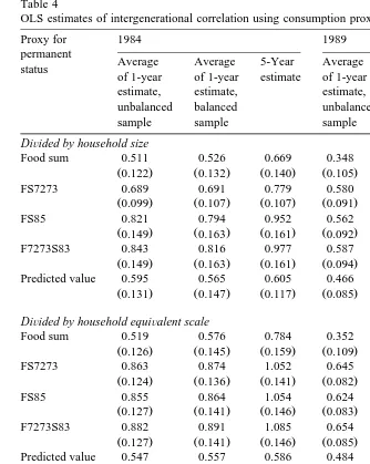
Table 4 presents the OLS estimates of the intergenerational coefficient when the various consumption measures are used to proxy for the sons’ and fathers’ statuses and when different methods are used to adjust for household size and structure. Columns 1–3 use 1984 measures for the sons’ outcomes. The first column presents the average estimates where the status of fathers is measured
Ž .
using a single year of data 1967–1971 and the unbalanced sample is used. The second column reports the average correlation estimate when fathers’ status is measured in a single year and the balanced sample is used. The third column of Table 4 reports the estimates when the father’s status is proxied by a 5-year average of the measure of his status. Columns 4–6 are analogous to columns 1–3 but use the 1989 measures of the sons’ outcomes.
In Table 4, the top five rows present the results when the proxies used are divided by household size. The second five rows divide the proxies by a household equivalent scale to adjust for household size and structure. The bottom five rows do not account for household size or structure.
The estimates of intergenerational correlation in columns 1–3 of Table 4 point to greater persistence in status and well-being than was implied by the earnings data. When the food sum is used to proxy for socioeconomic status, the average correlation estimates using a single year of data on fathers are approximately 0.5 and 0.6 for the unbalanced and balanced samples across the different methods of treatment for household size and structure. Using the weighted sum of the four components of consumption produces estimates of the correlation between fathers’ and sons’ statuses that are considerably higher. The single-year estimates using the weighted sums as proxies for permanent status range from 0.689 to 0.934 for the unbalanced sample and 0.691 and 0.891 for the balanced sample. The correlation estimates using the predicted value to proxy for status are lower, with the correlation estimates ranging from 0.423 to 0.595 for the unbalanced sample and from 0.506 to 0.565 for the balanced sample.
Table 4
OLS estimates of intergenerational correlation using consumption proxies for permanent status
Proxy for 1984 1989
permanent
Average Average 5-Year Average Average 5-Year
status
of 1-year of 1-year estimate of 1-year of 1-year estimate
estimate, estimate, estimate, estimate,
unbalanced balanced unbalanced balanced
sample sample sample sample
DiÕided by household size
Food sum 0.511 0.526 0.669 0.348 0.310 0.403
Ž0.122. Ž0.132. Ž0.140. Ž0.105. Ž0.107. Ž0.113.
FS7273 0.689 0.691 0.779 0.580 0.588 0.674
Ž0.099. Ž0.107. Ž0.107. Ž0.091. Ž0.099. Ž0.099.
FS85 0.821 0.794 0.952 0.562 0.569 0.657
Ž0.149. Ž0.163. Ž0.161. Ž0.092. Ž0.101. Ž0.100.
F7273S83 0.843 0.816 0.977 0.587 0.593 0.684
Ž0.149. Ž0.163. Ž0.161. Ž0.094. Ž0.103. Ž0.102.
Predicted value 0.595 0.565 0.605 0.466 0.468 0.506
Ž0.131. Ž0.147. Ž0.117. Ž0.085. Ž0.101. Ž0.079. DiÕided by household equiÕalent scale
Food sum 0.519 0.576 0.784 0.352 0.328 0.473
Ž0.126. Ž0.145. Ž0.159. Ž0.109. Ž0.107. Ž0.116.
FS7273 0.863 0.874 1.052 0.645 0.658 0.781
Ž0.124. Ž0.136. Ž0.141. Ž0.082. Ž0.093. Ž0.097.
FS85 0.855 0.864 1.054 0.624 0.637 0.766
Ž0.127. Ž0.141. Ž0.146. Ž0.083. Ž0.095. Ž0.098.
F7273S83 0.882 0.891 1.085 0.654 0.666 0.799
Ž0.127. Ž0.141. Ž0.146. Ž0.085. Ž0.097. Ž0.101.
Predicted value 0.547 0.557 0.586 0.484 0.487 0.537
Ž0.113. Ž0.129. Ž0.106. Ž0.078. Ž0.095. Ž0.076. No adjustment for household size or structure
Food sum 0.451 0.568 0.811 0.327 0.360 0.585
Ž0.140. Ž0.159. Ž0.182. Ž0.119. Ž0.110. Ž1.124.
FS7273 0.934 0.823 1.010 0.716 0.754 0.956
Ž0.110. Ž0.127. Ž0.131. Ž0.087. Ž0.100. Ž0.102.
FS85 0.720 0.812 1.012 0.689 0.726 0.942
Ž0.137. Ž0.131. Ž0.137. Ž0.087. Ž0.097. Ž0.103.
F7273S83 0.747 0.839 1.047 0.720 0.757 0.979
Ž0.112. Ž0.132. Ž0.137. Ž0.089. Ž0.104. Ž0.106.
Predicted value 0.423 0.506 0.526 0.504 0.526 0.617
Ž0.121. Ž0.141. Ž0.114. Ž0.086. Ž0.102. Ž0.080. Ž .
Standard errors SE are in parentheses. Sample sizes vary in the unbalanced sample. The sample size for the balanced and the 5-year samples is 254.
consumption are substantially lower when the 1989 measures vs. the 1984 measures are used to proxy for sons’ status. When the food sum is used to measure status, the estimates of the correlation between sons’ outcomes and their fathers’ average outcomes over the years 1967–1971 lie near 0.4. When the weighted sums are used to measure status, the estimates of the intergenerational coefficient range from about 0.7–1.0. When the predicted values are used to measure status, the estimates of the correlation are in the neighborhood of 0.5.
When either the sons’ 1984 or 1989 measures are used, the estimates where consumption is divided by family size are the smallest. The estimates where no account of family size is taken are greater than those that use an adult equivalent scale. When the sons’ 1989 measures are used and when either the household equivalent scale is used or the measures are divided by family size, the estimated correlations between fathers’ and sons’ consumption proxies are smaller and more similar to the estimates from the earnings data. This is not the case when 1984 consumption measures are used.
Additional research is required to explain why the estimates using consumption data lie above the estimates that use earnings to measure economic status. The higher transmission of consumption measures may be a result of the transmission of saving behavior or intra-familial transfers. Alternatively, the consumption measures used here may overstate the transmission of status if the intergenera-tional correlation in one of the components of the consumption proxies exceeds the degree of transmission of consumption overall. This paper does not examine these issues.
4. Conclusion
The estimates of the correlation between fathers’ and sons’ earnings lie in the neighborhood of 0.4. This is the case when I attempt to replicate Solon’s work and when son’s earnings from 5 years later are used in the estimation.
The estimates of the correlation between father’s and son’s consumption—using various proxies for consumption—are larger. The estimates of the consumption correlations are sensitive to whether son’s 1984 or 1989 outcomes are employed and whether one adjusts for household size and structure. The estimates of the intergenerational coefficient using 1984 sons’ outcomes are between 0.6 and 1.0. Using the later consumption measures to proxy for the status of the sons’ results in lower estimates of the correlation between fathers’ and sons’ statuses that are between 0.4 and 0.9.
Ž .
Acknowledgements
I thank David Blau, Sandy Darity, Greg Duncan, Donna Gilleskie, Tom Mroz, Gary Solon, and two anonymous referees for helpful comments on previous drafts. All errors are, of course, my own. The views of this paper do not represent those of the Bureau of Labor Statistics or its staff members.
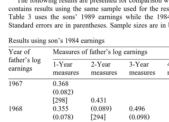
Appendix A. Results using 1989 sample and 1984 measures
The following results are presented for comparison with Table 3. This appendix contains results using the same sample used for the results in Table 3. However, Table 3 uses the sons’ 1989 earnings while the 1984 earnings are used here. Standard errors are in parentheses. Sample sizes are in brackets.
Results using son’s 1984 earnings
Year of Measures of father’s log earnings father’s log
1-Year 2-Year 3-Year 4-Year 5-Year earnings
measures measures measures measures measures
1967 0.368
Ž0.082.
w298x 0.431
Ž .
1968 0.355 0.089 0.496
Ž0.078. w294x Ž0.098.
w294x 0.389 w262x 0.503
Ž . Ž .
1969 0.258 0.085 0.469 0.099 0.455
Ž0.067. w262x Ž0.093. w259x Ž0.097. w264x 0.422 w259x 0.424 w254x
Ž . Ž .
1970 0.283 0.086 0.366 0.092
Ž0.069. w261x Ž0.086. w254x w294x 0.276 w256x
Ž .
1971 0.167 0.075
Ž0.061. w288x w288x
References
Altonji, J.G., Hayashi, F., Kotlikoff, L., 1992. Is the extended family altruistically linked? Direct evidence using micro data. American Economic Review 82, 1177–1198.
Becker, G.S., Mulligan, C.B., 1997. On the endogenous determination of time preferences. The Quarterly Journal of Economics 112, 729–758.
Becker, G.S., Tomes, N., 1986. Human capital and the rise and fall of families. Journal of Labor Economics 4, S1–S39.
Couch, K.A., Dunn, T.A., 1997. Intergenerational correlations in labor market status: a comparison of the United States and Germany. Journal of Human Resources 32, 210–232.
Couch, K.A., Lillard, D.R., 1998. Sample selection rules and the intergenerational correlation of earnings. Labour Economics 5, 313–329.
Dearden, L., Machin, S., Reed, H., 1997. Intergenerational mobility in Britain. Economic Journal 107, 47–66.
Fitzgerald, J., Gottschalk, P., Moffitt, R., 1998. An analysis of the impact of sample attrition on the second generation of respondents in the Michigan panel study of income dynamics. Journal of Human Resources 33, 300–344.
Lazear, E.P., Michael, R.T., 1988. Allocation of Income Within the Household. Univ. of Chicago Press.
Lillard, L.A., Kilburn, M.R., 1997, Assortative mating and family links in permanent earnings. Mimeo, RAND.
McGarry, K., 1997, Intervivos transfers and intended bequests, NBER Working Paper No. 6345. McGarry, K., Schoeni, R.F., 1996. Transfer behavior with the family: results from the asset and health
dynamics survey. Journals of Gerontology 52B, 82–92.
McGarry, K., Schoeni, R.F., 1997. Transfer behavior: measurement and the redistribution of resources within the family. Journal of Human Resources 30, S184–S226.
Mulligan, C.B., 1997. Parental Priorities and Economic Inequality. Univ. of Chicago Press.
Reville, R.T., 1995. Intertemporal and life cycle variation in measured intergenerational earnings mobility. Mimeo, Brown University.
Skinner, J., 1987. A superior measure of consumption for the panel study of income dynamics. Economics Letters 23, 214–216.
Solon, G., 1992. Intergenerational income mobility in the United States. American Economic Review 82, 393–408.