Directory UMM :Data Elmu:jurnal:E:Economics Letters:Vol70.Issue2.Feb2001:

Abstract

We demonstrate that two popular measures of inequality related to the discussion of s_{-convergence lead to}

different conclusions when used on data from Penn World Table. The reason is that the measures assign different weights to individual countries’ growth performance.  2001 Elsevier Science B.V. All rights reserved.

Keywords: Economic growth; Convergence

JEL classification: O40; O50

1. Two measures of s-convergence

Barro and Sala-i-Martin (1992) introduced the notion ofs_{-convergence.} s_{-convergence is said to}

be present if the dispersion of income per capita (or worker) across countries, measured by some convenient measure of dispersion, display a tendency to decline through time. Two popular measures of dispersion used in this context are (i) the coefficient of variation, c, and (ii) the standard deviation of log income per worker, v, i.e.:

*Corresponding author. Tel.: 1_{45-35-323-055; fax:} 1_{45-35-323-000.}

E-mail address: carl.johan.dalgaard@econ.ku.dk (C.-J. Dalgaard).

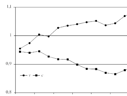
Fig. 1. The figure shows the standard deviation of log income and the coefficient of variation for 121 countries. The income measure used is GDP per worker. Datasource: Penn World Table.

1

As is well known, v and c have been used interchangeably in the literature on convergence. To the

extent that income across countries is lognormally or Pareto distributed then the two measures are indeed equivalent, in the sense that they both will be increasing in inequality, measured by the variance or ‘Pareto’sa_{’, respectively (see e.g. Cowell, 1995, chapter 4). However, this may not be the}

case empirically. To apply these two measures on a cross section of countries we use data from Penn World Table (see Summers and Heston, 1991). Specifically we were able to construct a data set encompassing 121 countries with complete time series coverage of GDP per worker from 1960 to

2

1988. As is shown in Fig. 1, the startling finding is that the two measures diverge!

Hence, we either confirm or refute s_{-convergence depending on the measure used. Why is that?}

2. Why do the measures diverge?

To answer this question, one needs to start by considering the dynamics of the global income distribution over the past 30 years. The general pattern identified by e.g. de la Fuente (1997) and Durlauf and Quah (1998) is the tendency for the distribution to exhibit ‘Twin Peaks’. This means that countries situated at the bottom of the distribution in 1960, to a rough approximation, have grown poorer relative to the mean during the next 29 years. The ‘middle-class’ of 1960, however, has grown comparatively faster than the top quintile of 1960. Hence, whereas there has been a tendency to divergence between the poorest and the richest countries, there has been considerable convergence between the middle and the top of the world distribution of income. Therefore, the reason for c andv

to ‘diverge’ may simply be, that they attache different weights to these movements. To follow up on

1

Barro and Sala-i-Martin (1995) usevto examine convergence across US states and Japanese prefectures, whereas e.g. de

la Fuente (1997) uses bothvand c in his survey of the convergence literature.

2

1 i

general, however, growth rates can be expected to differ across countries. As is clear from Eqs. (3)

~ ~

and (4), c andv are determined as a weighted sum of the n growth observations. Most importantly,

the weights assigned to the n growth observations, by the respective measures, are markedly different.

i

To investigate whether the differences in weights can explain the puzzle, note at the outset that w and_c

i i

wv differ in two crucial respects. First, while wv is zero for the country with (geometric) mean

i i

income, w is negative for the country with (arithmetic) mean income. To be precise, w 5_{0 if}

c c

yi 2

] 5₁1_{c . As middle income countries have tended to grow relatively fast, this would clearly tend}

¯y

to bias the weighted sum in Eq. (3) downward.

i i

Second, w

u u

v is likely to be larger than w , if y is smaller than the relevant mean, and vice versa.

u u

c i _{y y}

i i

i _] i _]

This follows from the fact that w is a convex function of_{c ¯} while w is a concave function of_c .

*

y y

This is important, as the countries at the bottom the distribution have grown relatively slow. If the two measures of inequality place different weights on this fact, it may explain, in part, why the measures lead to different conclusions regarding s_{-convergence.}

i i

To see that these differences between w and w are in fact non-negligible, a numerical example isc v

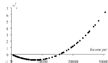
illustrative. In Figs. 2 and 3, the weights assigned to the 121 countries growth performance, by the two measures, are computed for 1970.

i i

As can be seen from visual inspection of Figs. 2 and 3, w and w change sign at very different_c v

i

levels of income. While w is negative for all countries with income levels below US$ 5309 (thev

i

geometric mean), w turns positive at US$ 15531. This means, in terms of the sample at hand, that nov

less than 40 growth observations are attached with weights of different sign by the respective

i i

measures; while w is positive, w is negative. As middle income countries on average have grownv c

comparatively fast, this bias would motivate why c declines while v increases, during the period

1960–1988.

Additionally, it is also apparent from the two figures that the two inequality measures place very different relative weights on the growth performance of economies placed at the bottom and the top of distribution of GDP per worker. As an illustration of the magnitudes involved, consider the weight on

3

~

i

Fig. 2. The figure shows w and income per worker for 121 countries in 1970. Datasource: Penn World Table.c

the richest economy relative to the poorest country which is implied by the two measures. In 1970 the richest country in the world was the United States with an annual PPP adjusted GDP per worker of 30 468 US$. At the other end of the spectrum Burundi was the poorest with an annual income per worker of only 590 US$. Computing the relative weights assigned to these two economies by the

us Burundi

respective measures (i.e. w /w , j5v, c), reveal that the coefficient of variation places 52

j j

times greater emphasis on the US growth rate, while the comparable number is 0.8 for the standard deviation of log income.

3. Conclusion

Although the variance of log income and the coefficient of variation are often regraded as equivalent measures of dispersion, they differ because of the weight assigned to the growth observations of the countries in the sample. Interestingly, this (at first glance) subtle difference is enough for the two measures to ‘diverge’ when used on a 121-country sample from Penn World Table.

By now, a vast literature exists on how to measure income inequality at any given point in time.

i

References

Barro, R., Sala-i-Martin, X., 1992. Convergence. Journal of Political Economy 100, 223–251. Barro, R., Sala-i-Martin, X., 1995. Economic Growth. McGraw-Hill, New York.

Cowell, F., 1995. Measuring Income Inequality. Prentice Hall, Englewood Cliffs, NJ.

Jones, C.I., 1997. On the evolution of the world income distribution. Journal of Economic Perspectives 11, 19–36. Lambert, P.J., 1993. The Distribution and Redistribution of Income — A Mathematical Analysis. Manchester University

Press, Manchester.

de la Fuente, A., 1997. The empirics of growth and convergence: A selective review. Journal of Economic Dynamics and Control 21, 23–73.

Durlauf, S., Quah, D., 1998. The new empirics of economic growth. In: Handbook of Macroeconomics. CEP Discussion Paper no. 384.