www.elsevier.com/locate/dsw
Approximating separable nonlinear functions via mixed zero-one
programs
Manfred Padberg
1Room 710, Operations Management Department, New York University, 40 West 4th Street, New York, NY 10003, USA
Received 1 February 1999; received in revised form 1 January 2000
Abstract
We discuss two models from the literature that have been developed to formulate piecewise linear approximations of separable nonlinear functions by way of mixed-integer programs. We show that the most commonly proposed method is computationally inferior to a lesser known technique by comparing analytically the linear programming relaxations of the two formulations. A third way of formulating the problem, that shares the advantages of the better of the two known methods, is also proposed. c 2000 Elsevier Science B.V. All rights reserved.
Keywords:Nonlinear functions; Piecewise linear approximation; Mixed-integer programming; Locally ideal formulations
1. Introduction
Applications of linear programming technology of-ten require the modeling of nonlinearities in the objec-tive function or in some of the constraints of an oth-erwise linear optimization model. Such nonlinearities may come about due to economies or diseconomies of scale, “kinked” demand or production cost curves, etc. Already in the early 1950s it has been recognized that such occurrences can be dealt with adequately by approximating nonlinearities by piecewise linear func-tions and modeling these in a mixed-integer frame-work by introducing new 0 –1 variables; see e.g. [1]
1Supported in part by a grant from the Oce of Naval Research (N00014-96-0327). Work done in part while visiting IASI-CNR in Rome, Italy, and the Forschungsinstitut fur Diskrete Mathematik, Universitat Bonn, Germany.
for an overview and historical references. Most text-books in Operations Research=Integer Programming, see e.g. [3,7] and others, oer one or two possibili-ties of expressing piecewise linear approximations of separable nonlinear functions in this manner.
The two classical formulations (Models I and II, below) can be found, e.g., in [2]. We are, however, not aware of a discussion of thequalityor tightness
of the various formulations that have been proposed a long while ago. Such considerations play indeed an essential role when the resulting mixed 0 –1 pro-gram is subsequently solved by branch-and-bound or branch-and-cut using linear programming algorithms (see e.g. [4]) in the solution process.
Besides reviewing the two classical formulations, the issue of the quality of the formulation is what we address here. We show that an analytical compari-son of the two dierent formulations of the problem
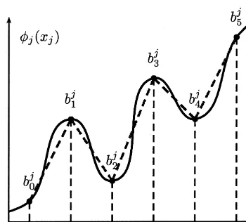
Fig. 1. Piecewise linear approximation.
reveals that one of them is always inferior to the other, i.e., the linear programming relaxation produces al-waysworse bounds in one case than in the other. We then propose a third way of formulating piecewise linear approximation via a mixed 0 –1 program that shares the (local) properties of the better of the two classical formulations.
Let(x1; : : : ; xn) be any separable, nonlinear
func-tion fromRn into R. Separability means that we as-sume that the function can be written as
(x1; : : : ; xn) = n
X
j=1
j(xj); (1)
where eachj(xj) mapsRintoR. Given nite
inter-vals [a0j; auj] for each variablexj wherej∈ {1; : : : ; n}
we approximate each j(xj) by a piecewise linear
function ˆj(xj) over this interval. To do so we choose
a partitioning a0j¡ a1j¡ a2j¡· · ·¡ akjj =auj of the
interval [a0j; auj] for eachj∈ {1; : : : ; n}, see Fig. 1. It
is well known that by rening the partitioning, i.e., by choosingkjlarge enough and the distance between
any two consecutive points of the partitioning small enough, we can – under certain technical conditions – approximatej(xj) arbitrarily closely by such
piece-wise linear functions. We denote by
b‘j=j(a‘j) for 06‘6kj; (2)
the function values at the pointsa‘jwhich we can cal-culate wherej∈ {1; : : : ; n}. In the following, we drop the indexjfor notational convenience because we will
consider a single term of the right-hand side of (1) only. Of course, as there are typically constraints link-ing the variablesx1; : : : ; xnour proceeding is a “local”
analysis. What we are looking for is a “locally ideal” formulation of the approximation problem, i.e., a for-mulation that in the absence of other constraints mod-els the problem perfectly; see [5] for more detail.
2. The rst model
In Model I we write for the single, continuous vari-ablex
x=a0+y1+· · ·+yk:
We require that eachy‘ is a continuous variable
sat-isfying
(i) 06y‘6a‘−a‘−1 for 16‘6k and moreover, the following dichotomy:
(ii) for 16‘6k−1 eitheryi=ai−ai−1for 16i6‘ ory‘+1= 0:
Assuming that this can be “formulated” conve-niently, we then get the piecewise linear approxima-tion for any term of the right-hand side of (1) by way of
ˆ
(x) =b0+
b1−b0
a1−a0
y1+
b2−b1
a2−a1
y2
+· · ·+bk−bk−1
ak−ak−1
yk:
From (i) it follows that (ii) can be replaced by the requirement
(ii′) for 16‘6k −1 either y
i¿ai −ai−1 for 16i6‘ory‘+160:
To formulate this in linear inequalities using integer variables we introduce 0 –1 variablesz‘ and consider
the mixed 0 –1 model
x=a0+
k
X
‘=1
y‘; ˆ(x) =b0+
k
X
‘=1
b‘−b‘−1
a‘−a‘−1
y‘;
(3)
y16a1−a0; yk¿0; (4)
y‘¿(a‘−a‘−1)z‘; y‘+16(a‘+1−a‘)z‘
for 16‘6k−1; (5) where z‘∈ {0;1} for 16‘6k −1 are the “new”
0 –1 variable and (3), (4) describe the linear approx-imation correctly. Fork= 2 the correctness follows by examining the two cases where z1= 0 and 1, re-spectively. The correctness of the mixed 0 –1 model (3) – (5) for the piecewise linear approximation of a nonlinear function follows by induction onk.
It follows from (5) that every solution to (4) and (5) satises automatically
1¿z1¿z2¿· · ·¿zk−1¿0;
thus the upper and lower bounds on the 0 –1 variables are not required in the formulation. In a computer model, however, we would declare the variables
z‘ to be “binary” variables rather than general
“in-teger” variables. A similar remark applies to the 0 –1 variables of the second and third model be-low. In Theorem 1 (below) we prove that Model I is a locally ideal formulation for piecewise linear approximation.
3. The second model
In Model II – which is the only one that one nds, e.g., in [3] – we exploit the fact that given a partitioning a0¡ a1¡· · ·¡ ak = au every real
x∈[a0; au] can be written uniquely as a convex
com-bination of at most two consecutive points a‘; a‘+1 of the partitioning. Thus we write for the continuous variablex
x=a00+a11+· · ·+akk;
where we require that the continuous variables‘
sat-isfy
(i)Pk‘=0‘= 1; ‘¿0 for 06‘6k;
(ii) at most two consecutive‘ and‘+1, say, are
positive.
If requirement (ii) can be expressed conveniently using integer variables, we then get the piecewise lin-ear approximation for any term of the right-hand side of (1) by way of
ˆ
(x) =b00+b11+· · ·+bkk:
To formulate (i) and (ii) as the set of solutions to a mixed 0 –1 program we introduce 0 –1 variables‘for
06‘6k−1 and consider the model
–1 variables. Note that the nonnegativity of 0 and
k−1 is implied by (7). For k= 1 the formulations (6) – (9) of the problem at hand is evidently correct. The correctness of Model II for arbitraryk¿1 follows inductively.
4. Comparison of Models I and II
In the following weassumethatk¿3, because for
k62 either model is locally ideal. Model I haskreal variables andk−1 0 –1 variables, while Model II has
k+ 1 real variables andk0 –1 variables. To compare the two models we use the Eqs. (8) to eliminate0 and0from the formulation. Using the variable trans-formation for the remaining continuous variables
y‘= (a‘−a‘−1)
k
X
j=‘
j for 16‘6k
and its inverse mapping that we calculate to be
j=
y1
a1−a0
− y2
a2−a1
61−
k−1 X
‘=2
‘;
y‘
a‘−a‘−1
− y‘+1
a‘+1−a‘
6‘−1+‘
for 26‘6k−1;
(13)
yk¿0; yk6(ak−ak−1)k−1; (14)
‘¿0 for 16‘6k−2; (15)
where ‘∈ {0;1} for 16‘6k−1. Note that (11)
implies thatPk−1
‘=1‘61 and thusP‘k=−j1‘61 for all
16j6k−1 and feasible 0 –1 values‘; 16‘6k−1.
Using the variable substitution
zj= k−1 X
‘=j
‘ for 16j6k−1;
which isintegrality preservingbecause its inverse is given by
j=zj−zj+1 for 16j6k−2; k−1=zk−1; the above constraints (11) – (15) can be written equiv-alently as follows:
y16a1−a0; y1¿(a1−a0)z1; (16)
(a‘−a‘−1)y‘+16(a‘+1−a‘)y‘ for 16‘6k−1;
(17)
y1
a1−a0
− y2
a2−a1
61−z2;
y‘
a‘−a‘−1
− y‘+1
a‘+1−a‘
6z‘−1−z‘+1
for 26‘6k−1;
(18)
yk¿0; yk6(ak−ak−1)zk−1; (19)
z‘−z‘+1¿0; for 16‘6k−2; (20) where for‘=k−1 we simply letzk=0 in (18) and the
integer variablesz‘ are 0 –1 valued for 16‘6k−1.
It follows that the (equivalently) changed Model II has now the same variable set as Model I and we are in the position to compare the two formulations in the context of a linear programming-based approach to the solution of the corresponding mixed-integer programming problem. Note that like in Model I the constraints (16), (19) and (20) imply that every
feasible solution to (16) – (20) automatically satises 1¿z1¿z2¿· · ·¿zk−1¿0.
We denote the linear programming (LP) relaxation of Model I by
FLPI ={(y;z)∈R2k−1: (y;z) satises (4) and (5)}: (21)
Likewise we denote the LP relaxation of the (equiva-lently) changed Model II by
FLPII ={(y;z)∈R2k−1:(y;z) satises (16)–(20)}: (22)
It is an immediate consequence of the respective for-mulations that bothFI
LP andFLPII areboundedsubsets and thus polytopes inR2k−1.
Theorem 1. (i) Model I is locally ideal, i.e.,
z∈ {0;1}k−1for all extreme points inFI LP. (ii)FI
LP is properly contained inFLPII: FLPII has
ex-treme points(y;z) withz6∈ {0;1}k−1.
Proof. We scale the continuous variables of Model I by introducing new variables
y′
‘=y‘=(a‘−a‘−1) for 16‘6k: (23) The constraint set deningFI
LPcan thus be written as
y′
161; y′k¿0; y′‘¿z‘; y′‘+16z‘ for 16‘6k−1:
(24)
It follows that the constraint matrix given by (24) is totally unimodular and hence by Cramer’s rule every extreme point of the feasible given by (24) has all components equal to zero or one. This implies (i).
(ii) Let (y;z)∈FI
LP, i.e., (y;z) satises (4) and (5). Then (y;z) satises (16) and (19) trivially. From (5) anda‘−a‘−1¿0 for all 16‘6kwe calculate (a‘+1−a‘)y‘¿(a‘+1−a‘)(a‘−a‘−1)z‘
¿(a‘−a‘−1)y‘+1
for 16‘6k−1 and thus (17) is satised. From (4) and (5) we havey16a1−a0andy2¿(a2−a1)z2and thus the rst relation of (18) follows. Again from (5) we havey‘6(a‘−a‘−1)z‘−1andy‘+1¿(a‘+1−a‘)z‘+1 for all 26‘6k−1, wherezk= 0, and thus
combin-ing the two inequalities we see that (18) is satised. As we have noted in the discussion of Model I ev-ery (y;z)∈FI
and thus (20) is satised as well. Consequently,
LP has extreme points with frac-tional components for z and indeed it has many such extreme points. It is not overly dicult to characterize all of them, which we leave as a good exercise for graduate students. It is amazing that most textbooks treat only Model II in the context of using mixed-integer programming to approximate separable nonlinear functions by piecewise linear ones.
Model I, which has been known since the 1950s, is
locallyfar better than Model II since all of its extreme points (y;z) satisfyz∈ {0;1}k−1. Of course, this does not mean that the “overall” model – of which the piece-wise linear approximation is but a part – has the same property. But the proper inclusion FI
LP⊂FLPII shows that the linear programming bound obtained from us-ing Model I must always be equal to or better than the one obtained from Model II in any case, i.e., even in theworstcase.
It is now an easy exercise to derive ex post a for-mulation of Model II in andvariables that guar-antees the same outcome as Model I. We leave it as an exercise to prove that the following Model III is a correct formulation, which is obtained from Model I by reversing the various transformations that we have used to analyze Model II:
x=
Evidently, Model III has at rst sight little resem-blance to the original Model II except that the same set of variables is used. More precisely, let
PLP={(;)∈R2k+1: (;) satises (7);(8);(9)};
P#LP={(;)∈R2k+1: (;) satises (26);(27);(28)};
be the linear programming relaxation of Models II and III, respectively. It follows that
P#LP⊂PLP and P#LP=conv(PLP∩(Rk+1×Zk)): By construction, Model III shareslocallythe property of Model I of having all its extreme points (;) sat-isfy∈ {0;1}k. Model III can be used in lieu of Model
I, but Model II should denitely be abandoned despite its popularity in the textbooks. Model II just happens to be a poor formulation for the piecewise linear ap-proximation problem when linear programming meth-ods are used. For more on analytical comparisons of dierent formulations of combinatorial optimization problems see e.g. [6].
References
[1] M.L. Balinski, K. Spielberg, Methods for integer programming: algebraic, combinatorial and enumerative, in: Aronofsky (Ed.), Progress in Operations Research, Wiley, New York, 1969, pp. 195 –292.
[2] G.B. Dantzig, Linear Programming and Extensions, Princeton University Press, Princeton, NJ, 1963.
[3] G. Nemhauser, L. Wolsey, Integer and Combinatorial Optimization, Wiley, New York, 1988.
[4] M. Padberg, Linear Optimization and Extensions, 2nd Edition, Springer, Heidelberg, 1999.
[5] M. Padberg, M. Rijal, Location, Scheduling, Design and Integer Programming, Kluwer Academic Publishers, Boston, 1996.
[6] M. Padberg, T.-Y. Sung, An analytical comparison of dierent formulations of the travelling salesman problem, Mathematical Programming 52 (1991) 315.