E l e c t r o n ic
J o ur n
a l o
f P
r o b
a b i l i t y
Vol. 10 (2005), Paper no. 2, pages 21-60.
Journal URL
http://www.math.washington.edu/∼ejpecp/
Convergence of Coalescing Nonsimple Random Walks to the Brownian Web C. M. Newman1 , K. Ravishankar2 and Rongfeng Sun3
Abstract
The Brownian Web (BW) is a family of coalescing Brownian mo-tions starting from every point in space and timeR×R. It was first
in-troduced by Arratia, and later analyzed in detail by T´oth and Werner. More recently, Fontes, Isopi, Newman and Ravishankar (FINR) gave a characterization of the BW, and general convergence criteria allowing in principle either crossing or noncrossing paths, which they verified for coalescing simple random walks. Later Ferrari, Fontes, and Wu verified these criteria for a two dimensional Poisson Tree. In both cases, the paths are noncrossing. To date, the general convergence cri-teria of FINR have not been verified for any case with crossing paths, which appears to be significantly more difficult than the noncrossing paths case. Accordingly, in this paper, we formulate new convergence criteria for the crossing paths case, and verify them for non-simple co-alescing random walks satisfying a finite fifth moment condition. This is the first time that convergence to the BW has been proved for mod-els with crossing paths. Several corollaries are presented, including an analysis of the scaling limit of voter model interfaces that extends a result of Cox and Durrett.
1
Research supported in part by NSF grant DMS-0104278
2
Research supported in part by NSF grant DMS-9803267
3
Keywords and Phrases: Brownian Web, Invariance Principle, Coalescing Random Walks, Brownian Networks, Continuum Limit.
1
Introduction and Results
The idea of the Brownian Web dates back to Arratia’s thesis [1] in 1979, in which he constructed a process of coalescing Brownian motions starting from every point in space R at time zero. In a later unpublished manuscript [2],
Arratia generalized this construction to a process of coalescing Brownian mo-tions starting from every point in space and timeR×R, which is essentially
what is now often called the Brownian Web (BW). He also defined a dual family of backward coalescing Brownian motions equally distributed (after a time reversal) with the BW which we call the Dual Brownian Web. Unfor-tunately, Arratia’s manuscript was incomplete and never published, and the BW was not studied again until a paper by T´oth and Werner [27], in which they constructed and analyzed versions of the Brownian Web and Dual Brow-nian Web in great detail and used them to construct a process they call the
True Self Repelling Motion.
In both Arratia’s and T´oth and Werner’s constructions of the BW, some semicontinuity condition is imposed to guarantee a unique path starting from every space-time point. More recently, Fontes, Isopi, Newman and Ravis-hankar [15, 16] gave a different formulation of the BW which provides a more natural setting for weak convergence, and they coined the term Brow-nian Web. Instead of imposing semicontinuity conditions, multiple paths are allowed to start from the same point. Further, by choosing a suitable topol-ogy, the BW can be characterized as a random variable taking values in a complete separable metric space whose elements are compact sets of paths. In [16], they gave general convergence criteria allowing either crossing or non-crossing paths, and they verified the criteria for the nonnon-crossing paths case for coalescing simple random walks. Recently, Ferrari, Fontes, and Wu [14] verified the same criteria for the noncrossing paths case for a two dimensional Poisson tree.
paths case, tightness needs to be checked separately. Furthermore, corre-lation inequalities in general no longer apply, and new ideas are needed to verify a key convergence criterion denoted (B2′), as formulated in [16]. For
co-alescing nonsimple random walks, criterion (B′
2) turns out to be particularly
difficult to verify (and this has not yet been done). Instead, we formulate an alternative criterion (E1), which we verify along with tightness and the
other convergence criteria. Thus the main contributions of this paper are contained in Sections 4 and 6 where tightness and criterion (E1) are verified.
The new convergence criteria and our approach in verifying them should serve as a paradigm for establishing the weak convergence of general models with crossing paths to the Brownian Web. A consequence of the weak convergence of coalescing nonsimple random walks to the Brownian web is that, for the dual one-dimensional voter model with initial condition 1’s on the negative axis and 0’s on the positive axis, the interface region evolves as a standard Brownian motion after diffusive scaling. This partially recovers and extends a result of Cox and Durrett [9], which required rather difficult calculations.
Coalescing Random Walks: Let Y, a random variable with distribution
µY, denote the increment of an irreducible aperiodic random walk onZ. We will always assume E[Y] = 0, E[Y2] = σ2 < +∞ throughout this paper,
unless a weaker hypotheses is explicitly stated. For our main result, we will also need E[|Y|5] < +∞. We are interested in the discrete time process of
coalescing random walks with one walker starting from every site on Z × Z (first coordinate space, second coordinate time). All walkers have i.i.d.
increments distributed asY, and two walkers move independently until they first meet, at which time they coalesce. The path of a random walk is defined to be the linear interpolation of the random walk’s position at integer times. Note that for non-simple random walks, two random walk paths can cross each other many times before they eventually coalesce. If Y were such that the random walks had period d 6= 1, as in the case of simple random walks whered= 2, then we would just haveddifferent copies of coalescing random walks on different space-time sublattices, none of which interacts with the other copies.
Let X1 (with distribution µ1) denote the random realization of such a
collection of coalescing random walk paths on Z×Z, and let Xδ (with
dis-tribution µδ), δ <1, beX1 rescaled with the usual diffusive scaling ofδ/σ in
space, δ2 in time. The main result of our paper (see Theorem 1.5 below) is
We remark that there are natural interacting particle systems constructed out of simple random walks, but still with paths crossing each other before eventual coalescence, for which the methods of this paper should be applica-ble to prove convergence to the BW. For example, there is a coalescing simple random walk model on the space time lattice Z×Z, dual to the Stepping
Stone Model with no mutation (see, e.g., [21, 28, 13]), which may be defined as follows. One walker starts from every site on the latticeZ×Z×{1,· · · , M},
where the first two coordinates are space and time, and the third coordinate can be regarded as the color. Each walker makes transitions on the space-time lattice as a simple random walk, and at every transition, a color is independently chosen from {1,· · · , M} with equal probability. Two walk-ers make their space-time transitions and choose their corresponding colors independently until after they meet at the same space-time site and choose the same color, at which time they coalesce. Projecting the random walk paths onto the space-time plane Z×Z, and restricting attention to random
walks on the even sublattice (i.e., (x, y)∈Z×Z withx+y even), we obtain
a system of coalescing simple random walks with crossing paths. A proof of convergence for this and other similar models to the BW would require verification of the hypotheses of Theorem 1.4 below (see also Remark 1.6).
Brownian Web: We recall here Fontes, Isopi, Newman and Ravishankar’s [15, 16] choice of the metric space in which the Brownian Web takes its values. Let ( ¯R2, ρ) be the completion (or compactification) ofR2under the metric
ρ, where
ρ((x1, t1),(x2, t2)) = ¯ ¯ ¯ ¯
tanh(x1)
1 +|t1| −
tanh(x2)
1 +|t2| ¯ ¯ ¯ ¯∨ |
tanh(t1)−tanh(t2)|. (1.1)
¯
R2 can be thought of as the image of [−∞,∞]×[−∞,∞] under the mapping
(x, t)Ã(Φ(x, t),Ψ(t))≡ µ
tanh(x)
1 +|t| ,tanh(t)
. (1.2)
Fort0 ∈ [−∞,∞], let C[t0] denote the set of functions f from [t0,∞] to
[−∞,∞] such that Φ(f(t), t) is continuous. Then define
Π = [
t0∈[−∞,∞]
C[t0]× {t0}, (1.3)
where (f, t0)∈Π represents a path in ¯R2 starting at (f(t0), t0). For(f, t0) in
equal to f(t0) fort < t0. Then we take
d((f1, t1),(f2, t2)) = (sup
t |
Φ( ˆf1(t), t)−Φ( ˆf2(t), t)|)∨ |Ψ(t1)−Ψ(t2)|. (1.4)
(Π, d) is a complete separable metric space.
Let now H denote the set of compact subsets of (Π, d), with dH the induced Hausdorff metric, i.e.,
dH(K1, K2) = sup
g1∈K1
inf g2∈K2
d(g1, g2)∨ sup
g2∈K2
inf g1∈K1
d(g1, g2). (1.5)
(H, dH) is also a complete separable metric space. Let FH denote the Borel
σ-algebra generated bydH.
Lemma 1.1 Assume E[|Y|] < +∞, then for any δ ∈ (0,1], the closure of
Xδ in (Π, d) is almost surely a compact subset of (Π, d).
Proof. We prove the lemma only for X1, since the proof for Xδ is identical.
Denote the image of X1 under the mapping (Φ,Ψ) by X1′. We will show the
equicontinuity of paths in X′
1. Note that by the properties of (Φ,Ψ), this
reduces to showing the equicontinuity of X′
1 restricted to any time interval
[Ψ(k),Ψ(k+ 1)] withk ∈Z, which we denote byX′
1| Ψ(k+1)
Ψ(k) . Similarly denote
the restriction ofX1to the time interval [k, k+1] byX1|kk+1. Note thatX1|kk+1 consists of line segments corresponding to random walks jumping from sites inZ at time k to sites inZ at time k+ 1. If X′
1| Ψ(k+1)
Ψ(k) is not equicontinuous,
then there would exist a sequence of random walk jumps from sitesxn→ −∞ to sites yn > L for some L ∈ R (or from xn → +∞ to yn < L). Since
E[|Y|] < +∞, using Borel-Cantelli, it is easily seen that this is an event
with probability 0, hence X′
1| Ψ(k+1)
Ψ(k) is almost surely equicontinuous, and this
proves the lemma.
Remark 1.1 Note that the closure ofXδ, which from now on we also denote
by Xδ, is obtained from Xδ by adding all the paths of the form (f, t) with
t ∈δ2Z∪{+∞,−∞}andf ≡+∞or f ≡ −∞. X
δ is then a(H,FH)-valued
random variable.
In [15, 16], the Brownian Web ( ¯W with measure µW¯) is constructed as a
Theorem 1.2 There is an (H,FH)-valued random variable W¯ whose distri-bution is uniquely determined by the following three properties.
(o) from any deterministic point(x, t)inR2, there is almost surely a unique
path Wx,t starting from (x, t).
(i) for any deterministic n,(x1, t1), . . . ,(xn, tn), the joint distribution of
Wx1,t1, . . . , Wxn,tn is that of coalescing Brownian motions (with unit
diffusion constant), and
(ii) for any deterministic, dense countable subset D of R2, almost surely,
¯
W is the closure in (H, dH) of {Wx,t : (x, t)∈ D}.
The (H,FH)-valued random variable ¯Win Theorem 1.2 is called the standard Brownian Web.
Convergence Criteria and Main Result: In [16], there was also given a set of general convergence criteria for measures supported on compact sets of paths which can cross each other. We now state these criteria as four conditions on our random variables Xδ.
(I1) There exist single path valued random variables θyδ ∈ Xδ, for y ∈ R2,
satisfying: for D a deterministic countable dense subset of R2, for any
de-terministic y1, . . . , ym ∈ D, θy1
δ , . . . , θ ym
δ converge jointly in distribution as
δ →0+ to coalescing Brownian motions (with unit diffusion constant)
start-ing at y1, . . . , ym.
Let ΛL,T = [−L, L]× [−T, T] ⊂ R2. For x0, t0 ∈ R and u, t > 0, let
R(x0, t0;u, t) denote the rectangle [x0−u, x0 +u]×[t0, t0 +t] in R2. Define
At,u(x0, t0) to be the event (in FH) that K (in H) contains a path
touch-ing both R(x0, t0;u, t) and (at a later time) the left or right boundary of
the bigger rectangle R(x0, t0; 17u,2t) (the number 17 is chosen to avoid
frac-tions later). Then the following is a tightness condition for {Xδ}: for every
u, L, T ∈(0,+∞),
(T1) ˜g(t, u;L, T)≡t−1lim sup
δ→0+
sup
(x0,t0)∈ΛL,T
µδ(At,u(x0, t0))→0 as t→0+
As shown in [16], if (T1) is satisfied, one can construct compact sets Gǫ ⊂ H for each ǫ >0, such that µδ(Gc
subsets of Π whose image under the map (Φ,Ψ) are equicontinuous with a modulus of continuity dependent on ǫ.
For K ∈ H a compact set of paths in Π, define the counting variable Nt0,t([a, b]) for a, b, t0, t∈R, a < b, t >0 by
Nt0,t([a, b]) = {y∈R| ∃x∈[a, b] and a path in K which touches
both (x, t0) and (y, t0+t)}. (1.6)
Let lt0 (resp. rt0) denote the leftmost (resp. rightmost) value in [a, b] with
some path in K touching (lt0, t0) (resp. (rt0, t0)). Also define N +
t0,t([a, b])
(resp. Nt−0,t([a, b])) to be the subset of Nt0,t([a, b]) due to paths in K that
touch (lt0, t0) (resp. (rt0, t0)). The last two conditions for the convergence of
{Xδ} to the Brownian Web are
(B1′) ∀β >0,lim sup δ→0+
sup t>β
sup t0,a∈R
µδ(|Nt0,t([a−ǫ, a+ǫ])|>1)→0 as ǫ→0 +
(B2′) ∀β >0,1
ǫ lim supδ→0+
sup t>β
sup t0,a∈R
µδ(Nt0,t([a−ǫ, a+ǫ])6=N +
t0,t([a−ǫ, a+ǫ])
∪N−
t0,t([a−ǫ, a+ǫ]))→0 as ǫ→0 +.
The general convergence theorem of [16] is the following, where we have replaced our family {Xδ} with δ → 0 by a general sequence {Xn} with
n →+∞:
Theorem 1.3 Let{Xn} be a family of(H,FH)valued random variables sat-isfying conditions(I1),(T1),(B1′)and(B2′), thenXn converges in distribution
to the standard Brownian Web W¯.
Condition (B′
1) guarantees that for any subsequential limit X of {Xn}, and for any deterministic pointy∈R2, there isµX almost surely at most one path
starting from y. Together with condition (I1), this implies that for a
deter-ministic countable dense set D ⊂R2, the distribution of paths inX starting
from finite subsets of D is that of coalescing Brownian motions. Conditions (B′
1) and (B2′) together imply that for the family of counting random variables
η(t0, t;a, b) = |Nt0,t([a, b])|, we have E[ηX(t0, t;a, b)] ≤ E[ηW¯(t0, t;a, b)] =
1 + √b−a
of coalescing random walks Xδ, we have not yet been able to verify condition (B2′), but an examination of the proof of Theorem 4.6 in [16] shows that we can also use the dual family of counting random variables
ˆ
ηX(t0, t;a, b) =|{x∈(a, b) | ∃ a path in X touching (1.7)
bothR× {t0} and (x, t0+t)}|.
By a duality argument [27] (see also [1, 2, 16]), ˆη and η − 1 are equally distributed for the Brownian Web ¯W. We can then replace (B2′) by
(E1) If X is any subsequential limit of {Xδ}, then ∀t0, t, a, b∈R with t > 0
and a < b,E[ˆηX(t0, t;a, b)]≤E[ˆηW¯(t0, t;a, b)] = b√−a
πt.
With this change, we immediately obtain our modified general convergence theorem,
Theorem 1.4 Let{Xn} be a family of(H,FH)valued random variables sat-isfying conditions(I1),(T1),(B1′)and(E1), thenXnconverges in distribution
to the standard Brownian Web W¯.
The main result of this paper is
Theorem 1.5 If the random walk incrementY satisfiesE[|Y|5]<+∞, then
{Xδ} satisfy the conditions of Theorem 1.4, and hence converges in distribu-tion to W¯.
Remark 1.6 The main difficulty lies in the verification of the tightness con-dition (T1) and condition (E1). Condition (E1) in our general convergence
result, Theorem 1.4, may seem strong since it requires an upper bound that is actually exact, but as we will show in our proof of(E1)for{Xδ}in Section 6,
all we need are the Markov property of the random walks and an upper bound of the type lim supδ↓0E[ˆηXδ(t0, t;a, b)] ≤ C for some finite C depending on t, a, b.
Remark 1.7 Recently, Belhaouari et al. [8] have succeeded in verifying a version of the tightness criterion (T1) in the context of voter model interfaces
In Section 2, we list some basic facts about random walks, then in sections 3 to 6, we proceed to verify condition (B1′), (T1), (I1) and (E1). In section
7, we present some corollaries for one dimensional coalescing random walks and the dual non-nearest-neighbor voter models. In particular, we prove that under the assumption E[|Y|5] < +∞, the point process at rescaled
time 1 of coalescing nonsimple random walks starting from (δ/σ)Z at time
0 converges weakly to the point process at time 1 of coalescing Brownian motions starting from Rat time 0. This extends a result of Arratia [1], and
it follows that the density of coalescing nonsimple random walks starting from Z at time 0 decays as 1/(σ√πt), extending a result of Bramson and
Griffeath [5]. Another corollary that follows from the convergence of the coalescing random walks Xδ to the Brownian Web is that, for the dual voter model φZ−
t (x) with initial configurationφ
Z−
0 (x)≡1 forx∈Z− andφ
Z−
0 (x)≡
0 forx∈Z+∪{0}, under diffusive scaling, the time evolution of the interface
between the all 0 region and the all 1 region converges in distribution to a Brownian motion starting from the origin at time 0. This partially recovers and also extends a result of Cox and Durrett [9], in which they proved that under the assumption E[|Y|3] <+∞, the interface region is of size O(1) as
t → +∞, and under diffusive scaling, the position at rescaled time 1 of the interface converges in distribution to a standard Gaussian. In Section 7, we also discuss how our proof can be modified to establish the weak convergence of continuous time coalescing nonsimple random walks to the Brownian Web.
2
Random Walk Estimates
In this section, we introduce some notation that will be used throughout the paper, and we list some basic facts about random walks that will be used in later sections. The results are all standard, but for self-containedness we include them here.
Given macroscopic space and time coordinates (x, t) ∈ R2, define their
microscopic counterparts before diffusive scaling by ˜t=tδ−2 and ˜x=xσδ−1.
Quantities such as ˜u,t˜0 are defined from u, t0 similarly. Since µδ and µ1 are
related by diffusive scaling, we will do most of our analysis using µ1, with
x, t, u, t0 for µδ replaced by ˜x,˜t,u,˜ ˜t0 for µ1.
LetξA
s denote the state at time sof a system of coalescing random walks starting from a subset A ⊂ Z×Z. In the special case when A = B × {t0}
for some B ⊂Z, we will denote it byξB,t0
denote it by ξB
s , as in the case of B = Z. We will use µ1(·) to denote the
probability of events for systems of coalescing random walks on Z×Zsince
they are marginals of X1.
Denote the linearly interpolated path of a random walk starting at some point (x, t0) ∈ Z× Z by πx,t0(s). Denote the event that a random walk
starting at (x, t0) stays inside the interval [a, b] containing x up to timet by
Bx,t0 [a,b],t.
Givenr ∈Z, define stopping times
τx,t0
r = inf{n ≥t0, n∈Z | πx,t0(n) =r}, (2.1)
τx,t0
r+ = inf{n ≥t0, n∈Z | πx,t0(n)≥r}. (2.2)
When the time coordinate in the superscripts of ξ, π, B, τ, τ+ is 0, we will
suppress it. We will use Px and Ex to denote probability and expectation
for a random walk process starting from x at time 0. Px,y and Ex,y will
correspond to two independent random walks starting at xand y at time 0. Recall that we always assume the random walk incrementY is distributed such that the random walk is irreducible and aperiodic with E(Y) = 0 and E[Y2]<+∞, unless a different moment condition is explicitly stated.
Lemma 2.1 Let πx, πy be two independent random walks with increment Y
starting at x, y ∈Z at time 0. Let τx,y be the integer stopping time when the
two walkers first meet, and let l(x, y) = supn∈[0,τx,y]|π
x(n)−πy(n)|. Then
τx,y and l(x, y) are almost surely finite.
Proof.Let ¯πy−x(n) = πy(n)−πx(n). Then ¯πy−x is an irreducible aperiodic symmetric random walk starting at y−xwith increment distributed asµY ∗
µ−Y. The lemma is simply a consequence of the recurrence of ¯πy−x, which requires less than a finite second moment of Y.
Lemma 2.2 Let πx, πy, τ
x,y be as in Lemma 2.1. Then Px,y(τx,y > t) ≤ C
√
t|x−y| for some constant C independent of t, x and y.
Proof. Let ¯πy−x(n) = πy(n)−πx(n) as in the proof of Lemma 2.1. Let ¯
Py−x denote probability for this random walk, and let ¯τ0y−x denote the first
integer time when ¯πy−x = 0. Then Px,y(τ
x,y > t) = ¯Py−x(¯τ0y−x > t). When
|x−y|= 1, it is a standard fact (see e.g. Proposition 32.4 in [24]) that this probability is bounded by √C
assume x < y, and regard πx and πy as a subset of the system of coalescing random walks ξ{x,x+1,...,y}. Then
Px,y(τx,y > t)≤µ1(|ξ{tx,...,y}|>1)
= µ1(
y−1 [
i=x
{τi,i+1 > t})≤(y−x)P0,1(τ0,1 > t)≤
C(y−x) √
t .
This establishes the lemma.
Lemma 2.3 Letu >0andt >0be fixed, and letπ(s) =π0,0(s)be a random
walk starting from the origin at time 0. Let u,˜ ˜t and the event B0
[−u,˜u˜],˜t be
defined as at the beginning of this section (note that they depend on δ), and let (B0
[−u,˜u˜],˜t)
c be the complement of B0
[−u,˜u˜],˜t. If Bs is a standard Brownian
motion starting from 0, then
0< lim δ→0+
P0((B0
[−u,˜˜u],˜t)
c) = P( sup s∈[0,t]|Bs|
> u)<4e−u
2 2t.
Proof. The limit follows from Donsker’s invariance principle [11] for random walks. The first inequality is trivial, and the second inequality follows from a well-known computation for Brownian motion using the reflection principle.
Lemma 2.4 Let u, t,u,˜ ˜t be as before. Let πx, πy and τ
x,y be as in Lemmas 2.1−2.2withx < y. Letτx,y,u˜+ be the first integer time whenπx(n)−πy(n)≥
˜
u. If E[|Y|3]<+∞, and δ is sufficiently small, we then have Px,y(τx,y,u˜+ <(τx,y∧˜t))< C(t, u)δ
for some constant C(t, u) depending only on t and u.
Proof. Let z = x−y < 0. Note that x, y, z are fixed while ˜u,˜t → +∞ as δ → 0. For the difference of the two walks ¯πz(n) = πx(n)−πy(n), we still denote the first integer time when ¯πz = 0 by ¯τz
0, and the first integer
time when ¯πz ≥u˜by ¯τz
˜
u+. Note we are using the bar ¯·to emphasize the fact
that we are studying the symmetrized random walks. The inequality then becomes
¯
First we will prove that, for δ sufficiently small,
If δ is sufficiently small, the last inequality is valid by Lemma 2.3. Also by Lemma 2.2,
together they give (2.4).
Lemma 2.5 Let πx be a random walk with increment Y starting from x < 0 at time 0. If E[Y2] < +∞, then the overshoot πx(τx
0+) has a limiting
distribution as x→ −∞. In terms of the ladder variable Z =π0(τ10+),
lim x→−∞P[π
x(τx
0+) = k] =
P[Z ≥k+ 1] E[Z] .
Proof.This is a standard fact from renewal theory, see e.g. Proposition 24.7 in [24].
Lemma 2.6 Let πx, Y and Z be as in the previous lemma. If E[|Y|r+2]<
+∞ for some r >0, then [πx(τx
0+)]r is uniformly integrable in x∈Z−, and
lim x→−∞
E£[πx(τx
0+)]r ¤
= 1
E[Z]
+∞
X
k=1
krP[Z ≥k+ 1]<+∞.
Proof. Note that if we letγx denote the random walk starting fromx <0 at time 0 with increment distributed asZ, thenγxsimply records the successive maxima of the random walk πx, and so the overshoots πx(τx
0+) and γx(τ0x+)
are equally distributed. By a last passage decomposition for γx,
P[γx(τx
0+) = k] =
−1 X
i=x
Gγ(x, i)P[Z =k−i]≤P[Z ≥k+ 1],
where Gγ(x, i) is the probability γx will ever visit i. Since E[|Y|r+2] <+∞ implies E[Zr+1] < +∞ (see e.g. problem 6 in Chapter IV of [24]), we have E£[πx(τx
0+)]r ¤
≤ P+k=1∞krP[Z ≥ k+ 1] < +∞, giving uniform integrability.
The rest then follows from Lemma 2.5 and dominated convergence.
Lemma 2.7 Let ξZ
n be a system of coalescing random walks starting from
every site on Z at time 0, whose random walk increments are distributed as
Y with E[Y2] < +∞. Then pn ≡ µ1(0 ∈ ξZ
n) ≤ √Cn for some constant C
independent of the time n.
Remark 2.1 The proof we present here is an adaptation of the argument used by Bramson and Griffeath [5] to establish similar upper bounds for con-tinuous time coalescing simple random walks in Zd, d≥ 2. In Corollary 7.1
below, we will prove that in factpn∼1/(σ√πn)asn →+∞under a stronger
Proof. Let BM = [0, M −1]∩ Z, and let en(BM) = E[|ξnZ ∩ BM|]. By translation invariance, en(BM) =pnM, and
en(BM)≤
X
k∈Z
E[|ξBM+kM
n ∩BM|] =
X
k∈Z
E[|ξBM
n ∩(BM +kM)|] =E[|ξnBM|].
Since M − |ξBM
n |is at least as large as the number of nearest neighbor pairs in BM that have coalesced by time n, we may take expectation and apply Lemma 2.2 to obtain
E[|ξBM
n |]≤M−(M−1)µ1(|ξn{0,1}|= 1)≤M−(M−1)(1−
C
√
n)<1+M C
√
n.
Thereforepn <1/M+C/√n. Since M can be arbitrarily large for any fixed
n, we obtain pn≤C/√n.
Lemma 2.8 For any A ⊂ Z, let ξnA be a system of discrete time coalescing
random walks on Z starting at time 0 with one walker at every site in A,
where all the random walks have increments distributed as some arbitrary
Z-valued random variable Y. Then for any pair of disjoint sets B, C ⊂ Z,
and for any time n≥0,
P(ξA
n ∩B 6=∅, ξAn ∩C6=∅)≤P(ξnA∩B 6=∅)P(ξnA∩C 6=∅). (2.5)
In particular, if x, y are any two distinct sites in Z, we have
µ1(x∈ξ
Z
n, y ∈ξ
Z
n)≤µ1(x∈ξ
Z
n)µ1(y ∈ξ
Z
n). (2.6)
Proof. The continuous time version of this lemma is due to Arratia (see Lemma 1 in [3]). Our proof for the discrete time case is an adaptation of Arratia’s proof for the continuous time case. Arratia’s proof uses a theorem of Harris [18], which breaks down for discrete time because there are transitions between states that are not comparable to each other. However, this can be easily remedied by using an induction argument.
We can assumeA, B, C are all finite sets, since otherwise we can approx-imate by finite sets, and the relevant probabilities will all converge. The main tool in the proof is the duality between coalescing random walks and voter models. For any pair of finite disjoint sets B, C ⊂ Z, let φB,C
n , with distribution νB,C
n , be a discrete time multitype voter model on Z defined as follows. The state space is X ={−1,0,1}Z
0,φB,C0 (x) = 0 ifx∈(B∪C)c; φB,C
{Yx,n}x∈Z,n∈N are i.i.d. integer-valued random variables distributed as Y.
LetEA+ ⊂X (resp.,EA−⊂X) be the event that some site inA is assigned the value +1 (resp., −1). Then by the duality between voter models and coalescing random walks (see, e.g., [22]), P(ξnA∩B =6 ∅) =νnB,C(E+
A),P(ξAn ∩
C 6=∅) =νB,C
n (EA−), and P(ξAn ∩B 6=∅, ξnA∩C 6=∅) =νnB,C(EA+∩EA−). The correlation inequality (2.5) then becomes
νB,C
n (EA+∩EA−)≤νnB,C(EA+)νnB,C(EA−). (2.7) We can define a partial order on the state space X by setting η ≤ ζ ∈ X
whenever η(x)≤ζ(x) for all x∈Zd.A functionf : X →Ris called
increas-ing (resp., decreasincreas-ing) if for any η≤ζ,f(η)≤f(ζ) (resp., f(η)≥f(ζ)). An event E is called increasing (resp., decreasing) if 1E is an increasing (resp., decreasing) function. Clearly, for finite A, 1E+
A is an increasing function and 1E−
A is a decreasing function. Inequality (2.7) will follow if we show that νB,C
n has the FKG property (see, e.g, [17, 22]), i.e., for any two increasing functions f and g,R
We prove this by induction. For any pair of finite disjoint setsB, C ⊂Z,
ν0B,C has the FKG property because the measure is concentrated at a single configuration. Observe that ν1B,C is a product measure and therefore also has the FKG property (this is the consequence of a simple special case of the main result of [17]). We proceed to the induction step, which is a fairly standard argument [19]. Assume that for all disjoint finite sets B and C, and for all 0 ≤ k ≤ n−1, νkB,C has the FKG property. Let us denote the collection of sites in ZwhereφB,C
n−1(x) = 1 by Bn−1, and where φB,Cn−1(x) =−1
by Cn−1. Then for any two increasing functions f and g, conditioning on
where we have used the FKG property for both νnB,C−1 and forνBn−1,Cn−1
1 , and
the observation that the conditional expectationsR
f dνBn−1,Cn−1
1 ,
R
gdνBn−1,Cn−1 1
conditioned on φB,Cn−1 are still increasing functions. Therefore νB,C
n also has the FKG property. This concludes the induction proof, and establishes the lemma.
Remark 2.2 Lemma 2.8 is also valid for random walks in Zd by the same
argument.
3
Verification of condition
(
B
1′)
Let’s fix t0, a∈ R, β > 0, t > β, ǫ > 0. Also fix a δ and let ˜t0,˜t,˜a and ˜ǫ be
defined from t0, t, a and ǫ by diffusive scaling. Then we have
µδ(|Nt0,t([a−ǫ, a+ǫ])|>1) =µ1(|Nt˜0,t˜([˜a−ǫ,˜a˜+ ˜ǫ])|>1).
If ˜t0 =n0 ∈Z, then the contribution toN is all due to walkers starting from
[˜a−˜ǫ,˜a+ ˜ǫ]∩Z at timen0. Thus we have
µ1(|Nn0,˜t([˜a−˜ǫ,˜a+ ˜ǫ])|>1) =µ1(|ξ[˜a−ǫ,˜˜a+˜ǫ]∩
Z,n0
n0+˜t |>1) ≤
⌊˜a+˜ǫ⌋−1 X
i=⌈˜a−ǫ˜⌉
µ1(|ξn{i,i0+˜+1t },n0|>1)
≤ 2˜ǫµ1(|ξ˜t{0,1},0|>1)≤2˜ǫ
C
√ ˜
t =
2Cσǫ
√
t <
2Cσǫ
√
β (3.1)
The first inequality follows from the observation that if the collection of walkers starting from [˜a−˜ǫ,˜a+ ˜ǫ]∩Z at n0 has not coalesced into a single
walker byn0+˜t, then there is at least one adjacent pair of such walkers which
has not coalesced by n0+ ˜t. The next inequality follows from Lemma 2.2.
Now suppose ˜t0 ∈ (n0, n0 + 1) for some n0 ∈ Z. Note that a walker’s
path can only cross [˜a −˜ǫ,˜a+ ˜ǫ]× {˜t0} due to the increment at time n0.
After the increment, at time n0 + 1, it will either land in [˜a−2˜ǫ,a˜+ 2˜ǫ], or
else outside that interval. In the first case, the contribution of the walker’s path to N is included in ξ˜t[˜a−2˜ǫ,˜a+2˜ǫ]∩Z,n0+1
0+˜t , the probability of which by our
previous argument is bounded by 4Cσǫ√
right of ˜a+ 2˜ǫ, or a walker in [˜a−ǫ,˜ +∞) jumps to the left of ˜a−2˜ǫ, the probability of which is bounded by
+∞
X
x=⌈˜a−˜ǫ⌉
P(Y ≤a˜−2˜ǫ−x) + ⌊˜a+˜ǫ⌋
X
x=−∞
P(Y ≥˜a+ 2˜ǫ−x)
≤
+∞
X
k=0
P(|Y| ≥k+ ˜ǫ) ≤
+∞
X
k=0
E[Y2,|Y| ≥k+ ˜ǫ]
(k+ ˜ǫ)2
≤
+∞
X
k=0
E[Y2,|Y| ≥˜ǫ]
(k+ ˜ǫ)2 ≤
2E[Y2,|Y| ≥˜ǫ]
˜
ǫ ≤
4σ2
˜
ǫ =
4σδ
ǫ . (3.2)
The next to last inequality in (3.2) is valid if we take δ to be sufficiently small. The bounds in (3.1) and (3.2) are independent of t0, t > β and a.
Taking the supremum over t > β, t0 and a, and letting δ → 0+, we obtain
(B1′).
Corollary 3.1 Assume X (with distribution µ) is a subsequential limit of
Xδ, then for any deterministic point y ∈ R2, X has almost surely at most
one path starting from y.
Proof. It was shown in the proof of Theorem 5.3 in [16] that (B′
1) implies
(B1′′) ∀β >0,sup t>β
sup t0,a∈R
µ(|Nt0,t([a−ǫ, a+ǫ])|>1)→0 as ǫ→0 +
and the corollary then follows.
Remark 3.1 Note that if ZAδ
δ is the process of coalescing random walks
starting from a subset Aδ of the rescaled lattice, and ZδAδ converges in
distri-bution to a limitZ, then by the same argument as above, for any deterministic point y∈R2, Z has almost surely at most one path starting from y.
4
Verification of tightness condition
(
T
1)
Define A+t,u(x0, t0) to be the event that K contains a path touching both
R(x0, t0;u, t) and (at a later time) the right boundary of the bigger rectangle
the left boundary of the bigger rectangle. Then A= (A+∪A−), and writing
(T1) in terms of µ1, we argue that it is sufficient to prove
(T1+) ˜g(t, u;L, T)≡t−1lim sup δ→0+
µ1(A+˜t,u˜(0,0)) →0 as t→0 +.
The sup over x0, t0 has been safely omitted because µ1 is invariant under
translation by integer units of space and time. When ˜x0,˜t0 ∈/ Z, we can
bound the probability from above by using larger rectangles with vertices in Z×Z and base centered at (0,0). Since the argument establishing the
analogous tightness condition (T1−) for the event A− is identical to that for
(T1+), (T1) follows from (T1+). In the ensuing discussions, we will simply write
A+t,u(0,0) as A+t,u or just A+, and R(0,0;u, t) as R(u, t).
Before we prove (T1+), and hence (T1), we introduce some simplifying
notation. Denote random walks starting at time 0 from x1 = ⌈3˜u⌉, x2 =
⌈7˜u⌉, x3 = ⌈11˜u⌉, x4 = ⌈15˜u⌉ by π1, π2, π3, π4. Denote the event that πi,
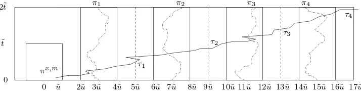
(i = 1,2,3,4) stays within a distance ˜u of xi up to time 2˜t by Bi (see Figure 1). For a random walk starting from (x, m) ∈ R(˜u,˜t), denote the integer stopping times that the walker first exceeds 5˜u,9˜u,13˜u and 17˜u by
τ1x,m, τ2x,m, τ3x,m and τ4x,m. We also define τ0x,m = m, and τ5x,m = 2˜t. Denote the event that πx,m does not coalesce with π
i before time 2˜t by Ci(x, m). As we shall see, the reason for choosing four paths πi is because each path contributes a factor of δ to our estimate of the µ1 probability in (T1+), and
an overall factor of δ4 is needed to outweigh the O(δ−3) number of lattice
points in the rectangle R(˜u,˜t) from where a random walk can start. We are now ready to prove (T1+).
Proof of (T1+). First we can assume ˜t ∈Z, since we can always replace
˜
t by ⌈˜t⌉ which only enlarges the event A+. The contribution to the event
A+ is either due to random walk paths that originate from withinR(˜u,˜t), or
paths that cross R(˜u,˜t) without landing inside it after the crossing. Denote the latter event by D(˜u,˜t). Then
µ1(A+˜t,u˜) ≤ µ1( 4 [
i=1
Bic) +µ1(D(˜u,t˜))
+ µ1( 4 \
i=1
Bi; ∃(x, m)∈R(˜u,˜t) s.t.
4 \
i=1
Ci(x, m), τ4x,m <2˜t). (4.1)
By Lemma 2.3, the first term on the right hand side of (4.1) is of order
14 ˜u
at time 0 and each stays within a distance of ˜u. The random walkπx,mstarts from (x, m) inside the rectangle R(0,0; ˜u,˜t) and exits the right boundary of
To estimate the third term in (4.1) (see Figure 1 for an illustration of the event), we first treat the case of a fixed (x, m)∈R(˜u,˜t). Suppressing (x, m)
The first part is bounded by
where ω(δ)→0 as δ →0. The last inequality is due to the uniform integra-bility of the third moment of the overshoot distribution, which follows from our assumption E[Y5]<+∞and Lemma 2.6.
For the second µ1 probability in (4.2), denote the event that none of the
conditions listed are violated by time t by Gt. If τ1 > t, we interpret an
inequality like π(τ1)≤521u˜as not having been violated by timet. Gt is then a nested family of events, and the second probability in (4.2) becomes
µ1(G2˜t) =µ1(Gτ5) = µ1(Gm)
and π4 up to time t by Πt, and denote expectation with respect to the
conditional distribution of Πt conditioned on the event Gt by Et. Then for
k = 1,2,3,4,
where the µ1 probability on the right hand side is conditioned on a given
realization of Πτk−1 ∈ Gτk−1, which is a positive probability event. For any
where the inequality follows from Lemma 2.4 for δ sufficiently small. Thus
Remark 4.1 The only place in this paper where we need the assumption
E[|Y|5]<+∞ is in (4.3). We needE[|Y|3]<+∞ to estimate µ1(D(˜u,˜t)) in
(4.1), and to apply Lemma2.4in (4.4). A finite third moment is the minimal moment condition for the convergence ofXδ. For anyǫ >0, there are choices
of Y satisfying E[|Y|3−ǫ] < +∞, but with µ1(D(˜u,t˜))→ 1 as δ → 0 for all
t >0, which implies {Xδ} is not tight.
5
Verification of condition
(
I
1)
Our verification of (I1) is essentially a careful application of Donsker’s
invari-ance principle and the Continuous Mapping Theorem for weak convergence. We define three sets of random walks: {πδ}i
1≤i≤m, a family of mindependent
random walks on the rescaled lattice (δ/σ)Z×δ2Z; {πi
δ,f}1≤i≤m, the family
of mcoalescing random walks constructed from {πiδ}by applying a mapping
f to {πδ}i ; and {πi
δ,g}1≤i≤m, an auxiliary family of m coalescing walks
con-structed by applying a mapping g to {πδ}i such that two walks coalesce as soon as their paths intersect (note that random walks in{πδ,g}i coalesce earlier than they do in{πi
δ,f}). By Donsker’s invariance principle,{πδ}i will converge weakly to a family of independent Brownian motions {Bi}
1≤i≤m. As we will
see, the mapping g is almost surely continuous with respect to {Bi}, and {Bg}i
1≤i≤m is distributed as coalescing Brownian motions. Therefore by the Continuous Mapping Theorem for weak convergence,{πδ,g}i converges weakly to the coalescing Brownian motions {Big}. Finally to show that {πi
δ,f} also converges weakly to {Bg}i , we will prove that the distance between the two versions of coalescing walks {πi
δ,f} and {πiδ,g} converges to 0 in probability. We start with some notation. LetDbe any deterministic countable dense subset of R2. Let y1 = (x1, t1), . . . , ym = (xm, tm) ∈ D be fixed, and let
B1, ...,Bm be independent Brownian motions starting from y1, ..., ym. For a fixedδ, denote⌈y˜i⌉= (⌈x˜i⌉,⌈˜ti⌉), where ˜xi =σδ−1xi and ˜t =δ−2ti as defined in Section 2, and letyi
δdenote⌈y˜i⌉’s space-time position after diffusive scaling on the rescaled lattice (δ/σ)Z×δ2Z. Let ˜πi (i = 1,· · · , m) be independent
random walks in the Z×Zlattice starting from⌈y˜i⌉. We regard (B1, ...,Bm),
and (˜π1, ...,π˜m) as random variables in the product metric space (Πm, d∗m), where
d∗m[(ξ1, . . . , ξm),(ζ1, . . . , ζm)] = max
1≤i≤m d(ξ
i, ζi) (5.1)
will also need the metric ¯
d((f1, t1),(f2, t2)) = sup
t | ˆ
f1(t)−fˆ2(t)| ∨ |t1−t2| (5.2)
and ¯d∗m is defined in a similar way as d∗m.
We now define a mappingg from (Πm, d∗m) to (Πm, d∗m) that constructs coalescing paths from independent paths. The construction is such that when two paths first intersect, the path with the higher index will be replaced by the path with the lower index after the time of intersection. This procedure is then iterated until no more intersections take place. To be explicit, we give the following algorithmic construction.
Let (ξ1, . . . , ξm) ∈ Πm, and start with equivalence relations on the set {1, . . . , m} by letting i ≁ j ∀ i 6= j. Define a one step iteration Γ on
(ξ1, . . . , ξm) and the equivalence relations by
τg = inf{t ∈R| ∃ i, j ∈ {1, . . . , m}, i≁j, ξi(t) =ξj(t)}, (5.3)
i∗ = min{j | 1≤j ≤m, ξi(τg) =ξj(τg)}, (5.4)
Γξi(t) =
½
ξi(t) if t≤τ g,
ξi∗
(t) if t > τg, (5.5)
and update equivalence relations by assigning i ∼ i∗. Iterate the mapping Γ, and label the successive intersection times τg by τgk. Then the iteration stops when τk
g = +∞ for some k ∈ {1,2, . . . , m}, i.e., either there is no more intersection among the different equivalence classes of paths, or all the paths have coalesced and formed a single equivalence class. Denote the final collection of paths by g(ξ1, . . . , ξm) = (ξ1
g, . . . , ξgm). Then it’s clear by the strong Markov property, that (B1
g, . . . ,Bmg ) has the distribution of coalescing Brownian motions. However (˜π1
g, . . . ,π˜gm) is not distributed as coalescing random walks, because for nonsimple random walks, paths can cross before the random walks actually coalesce (by being at the same space-time lattice site).
To construct coalescing random walk paths from independent random walks in Z×Z, we define another mapping f from (Πm, d∗m) to (Πm, d∗m)
in a similar way as we defined g, except in (5.3)–(5.5), the time of first intersection τg is replaced by the time of first coincidence on the unscaled lattice,
We will label the successive coincidence times byτk
f. Also denotef(ξ1,· · · , ξm) by (ξ1
f,· · · , ξfm). It is then clear that (˜πf1, . . . ,π˜mf ) is distributed as coalescing random walks starting from (⌈y˜1⌉, . . . ,⌈y˜m⌉) in the unscaled lattice Z×Z.
We shall denote the diffusively rescaled versions of (˜π1, . . . ,π˜m), (˜π1
g, . . . ,π˜mg ) and (˜π1
f, . . . ,π˜fm) by (πδ1, . . . , πδm), (πδ,g1 , . . . , πmδ,g) and (π1δ,f, . . . , πδ,fm). We need the following two lemmas to prove (I1).
Lemma 5.1 Let (B1, ...,Bm) be m independent Brownian motions starting
from (y1, ..., ym), and let (π1
δ, ..., πmδ ) be independent random walks starting
from (y1
δ, ..., yδm) in the rescaled lattice as defined before. Then (π1δ,g, ..., πδ,gm)
converges in distribution to (B1
g, ...,Bgm) as δ →0+. Proof. Clearly (y1
δ, . . . , yδm) converge to (y1, . . . , ym). By Donsker’s invari-ance principle [11], (π1
δ, ..., πmδ ) converges weakly to (B1, ...,Bm) as δ → 0+. From standard properties of Brownian motion, it is easy to see that the mapping g is almost surely continuous with respect to (B1, ...,Bm). Also note that (π1
δ,g, ..., πmδ,g) is the same as applyingg to (πδ1, ..., πδm), therefore by the Continuous Mapping Theorem for weak convergence (see, e.g., Section 8.1 of [12]), (π1
δ,g, ..., πδ,gm) converges in distribution to (B1g, ...,Bmg ) asδ →0+. Lemma 5.2 ∀ ǫ > 0, P{d∗m[(π1
δ,f, . . . , πmδ,f),(πδ,g1 , . . . , πmδ,g)] ≥ ǫ} → 0 as
δ →0+.
Proof. From the definition of d and ¯d in (1.4) and (5.2), it is clear that
d((f1, t1),(f2, t2))≤d¯((f1, t1),(f2, t2)) for any (f1, t1),(f2, t2)∈Π. Therefore
it is sufficient to prove the lemma with d∗m replaced by ¯d∗m. In terms of random walks in Z×Z, the lemma can be stated as
∀ ǫ >0,P{d¯∗m[(˜π1
f, . . . ,π˜fm),(˜π1g, . . . ,π˜mg )]≥˜ǫ} →0as δ →0+. (5.7) We first prove (5.7) for m = 2. Note that for m = 2, ˜π1
f = ˜π1g = ˜π1, hence ¯d∗2[(˜π1
f,π˜2f),(˜πg1,π˜g2)] = ¯d(˜π2f,˜π2g). Let ˜Tg1,2 denote the first integer time when ˜π1 and ˜π2 coincide or interchange relative ordering, and let ˜T1,2
f denote the first integer time when the two walks coincide. Also let l(0, n) denote the maximum distance over all time between two coalescing random walks starting at 0 and n at time 0. Then by the strong Markov property, and conditioning at time ˜T1,2
g ,
P[ ¯d(˜πf2,π˜g2) ≥ǫ˜]≤
+∞
X
n=1
The first probability in the summand converges to a limiting probability distribution as δ → 0 by applying Lemma 2.5 to (˜π1 −π˜2). The second
probability converges to 0 for every fixed nby Lemma 2.1. This proves (5.7) for m= 2.
For m > 2, let ˜Tfi,j and ˜Ti,j
g denote respectively the first integer time when the two independent walks ˜πi and ˜πj coincide or interchange relative ordering. As usual, let Tδ,fi,j = δ2T˜i,j
f and T i,j
δ,g = δ2T˜gi,j. Then by the weak convergence of (π1
δ,· · · , πδm) to (B1,· · · ,Bm) and the Continuous Mapping Theorem, {Tδ,gi,j}1≤i<j≤m converge jointly in distribution to{τi,j}1≤i<j≤m, the
associated pairwise first intersection times for{B1,· · · ,Bm}. By the standard properties of Brownian motion, {τi,j}
1≤i<j≤m are almost surely all distinct. By an argument similar to (5.8), we also have sup1≤i<j≤m|Tδ,fi,j −Tδ,gi,j| → 0 in probability. Note that in our definition of the mapping g that con-structs (˜π1
g,· · · ,π˜gm) from (˜π1,· · · ,˜πm), the successive times of intersection {τk
g}1≤k≤m−1, are all times of first intersection between independent paths,
i.e., {⌈τk
g⌉}1≤k≤m−1 ⊂ {T˜gi,j}1≤i<j≤m. The event in (5.7) can only occur due
to: either (1) for some τk
g in the definition of g, with ⌈τgk⌉ = ˜Tgi,j for some
i and j, τk+1
g ≤T˜ i,j
f ; or else, (2) whenever a coalescing takes place between two paths ˜πi,π˜j in the mapping g, the same two paths will coalesce in the mapping f before another coalescing takes place in the mapping g, and the event in (5.7) occurs because for some τk
g with ⌈τgk⌉= ˜Tgi,j, the distance be-tween the two paths ˜πi and ˜πj during the time interval [ ˜Ti,j
g ,T˜ i,j
f ] exceeds ˜
ǫ. The probability of the event (1) tends to 0 as δ →0 by our observations that {Tδ,gi,j}1≤i<j≤m converges jointly in distribution to {τi,j}1≤i<j≤m, which
are almost surely all distinct, and the fact that sup1≤i<j≤m|Tδ,fi,j −Tδ,gi,j| →0 in probability. The probability of the event (2) tends to 0 by our proof of (5.7) for m= 2. This proves (5.7) and Lemma 5.2.
Proof of (I1). Lemmas 5.1 and 5.2 imply that (πδ,f1 , . . . , πmδ,f) converge in distribution to (B1
g, ...,Bgm) asδ →0+ by converging together lemma (see, e.g., Section 8.1 of [12]). Certainly {π1
δ,f, . . . , πδ,fm} ⊂ Xδ, therefore (I1) is
6
Verification of condition
(
E
1)
As usual, we start with some notation. For an (H,FH)-valued random vari-able X, define Xs−
to be the subset of paths in X which start before or at times, and fors≤tdefineXs−,t
T to be the set of paths inXs− truncated be-fore time t, i.e., replacing each path inXs−
by its restriction to time greater than or equal to t. When s =t, we denote Xs−,s
We recall here the definition of stochastic domination as given in [16]. For two measures µ1 and µ2 on (H,FH), µ2 is stochastically dominated by
µ1 (µ2 << µ1) if for any bounded increasing function f on (H,FH), (i.e.
f(K)≤f(K′) ifK ⊂K′),Eµ
2[f]≤Eµ1[f]. Whenµ1, µ2 are the distributions
of two (H,FH)-valued random variables X1 and X2, we will also denote the
stochastic domination byX2 << X1. The first step of our proof is to reduce
(E1) to the following condition (E1′), which singles out the set of paths that
are of interest to us (i.e., the set of paths starting before time t0).
(E1′) IfZt0 is any subsequential limit of{X sequence δn ↓ 0. To prove the Lemma, it is sufficient to show that for any 0 < ǫ < t, there is a subsequence {δn}′ such that Xδ(′t0+ǫ)−
t0+ǫ, and the stochastic domination,
for all δn, {X(t0+ǫ)
−
δn } and {Wδn} are also tight. Therefore we can choose a subsequence δ′
n such thatWδ′
n converges weakly to a limitW. By Skorohod’s representation theorem (see, e.g., [4, 12]), we can define random variables
Wδ′′
with Lebesgue measure, such that they are equally distributed with Wδ′
n and W and the convergence of W′
δ′
0 is the limit of a sequence of paths
(fn, tn) ∈ Xδ′′ This finishes the proof of Lemma 6.1.
Condition (E′
1) would follow if we knew that asymptotically the density
of coalescing random walks is pn ∼ 1/(σ√πn) (see Lemma 2.7). But in the literature this result seems only to have been established for continuous time coalescing simple random walks. Instead of trying to directly establish the exact asymptotic density, we make the following observation. The coarse bound provided by Lemma 2.7 implies that Zt0(t0 +ǫ) is locally finite for
If we can verify that, which should be relatively easy because of the local finiteness of Zt0(t0 +ǫ), then condition (E1′) will follow since the system of
coalescing Brownian motions starting from a random locally finite set onRat
time t0+ǫ is certainly stochastically dominated by the system of coalescing
Brownian motions starting from every point on R at time t0 +ǫ, and for
the latter we know how to compute E[ˆη]. Sending ǫ to 0 will then establish
(E′
1). In Corollary 7.1 below, we will show that the convergence of Xδ to
the Brownian web also implies that the density of coalescing random walks is asymptotically 1/(σ√πn), so the coarse bound of Lemma 2.7 in fact leads to the exact asymptotics.
We now make everything precise. Let Zt0 be as in (E1′). (E1′) follows
from the next two lemmas, which are also what one needs to check in order to verify condition (E′
1) for general models other than coalescing random
walks.
Zt0 with the line t=t0+ǫ. Then for any ǫ >0, Zt0(t0+ǫ) is almost surely
locally finite.
Lemma 6.3 For any ǫ >0, Z(t0+ǫ)T
t0 , the set of paths in Zt0 (which all start
at time t ≤ t0) truncated before time t0+ǫ, is distributed as BZt0(t0+ǫ), i.e.,
coalescing Brownian motions starting from the random set Zt0(t0+ǫ)⊂R 2.
Proof of (E′
1). Assume Lemmas 6.2 and 6.3 for the moment. Since
BZt0(t0+ǫ) <<W¯, we have for 0< ǫ < t
E[ˆηZ
t0(t0, t;a, b)] = E[ˆη
Z(t0+ǫ)T
t0 (t0+ǫ, t−ǫ;a, b)] =
E[ˆη
BZt0(t0+ǫ)(t0+ǫ, t−ǫ;a, b)]
≤ E[ˆη¯
W(t0 +ǫ, t−ǫ;a, b)] =
b−a
p
π(t−ǫ) .
Since 0< ǫ < tis arbitrary, letting ǫ →0 establishes (E1′). Lemma 6.2 will be a consequence of the following: Lemma 6.4 ∀ t0, t, a, b∈R with t >0 and a < b, we have
lim sup δ→0+
E[ˆηX
δ(t0, t;a, b)]≤
C(b−a) √
t
for some 0< C <+∞ independent of t0, t, a and b.
Proof.By space-time lattice translation invariance and elementary argu-ments, we can assumet0 = 0 and (a, b) = (−r, r). Note thatE[ˆηXδ(0, t;−r, r)] =E[ˆηX
1(0,˜t;−r,˜ r˜)]. If ˜t∈Z, then
E[ˆηX
1(0,˜t;−r,˜ r˜)]≤(2˜r+ 1)µ1(0∈ξ
Z
˜
t) (6.1)
by translation invariance. If ˜t /∈Z, E[ˆηX
1(0,˜t;−r,˜ r˜)]
≤ E[ˆηX
1(0,⌊˜t⌋;−2˜r,2˜r) +
−2˜r
X
x=−∞
P(Y >−˜r−x) +
+∞
X
x=2˜r
P(Y <r˜−x)
≤ (4˜r+ 1)µ1(0∈ξ
Z
⌊˜t⌋) +
+∞
X
k=0
where by Lemma 2.7 the first quantity is bounded by (4˜r + 1)(C/p⌊˜t⌋), Define another counting random variable ˆη′
X(t0, t;a, b) = lims↓0ηˆX(t0−s, t+
Since a < b is arbitrary, the lemma then follows.
It only remains to prove Lemma 6.3. We need one more lemma. Denote the space of compact subsets of ( ¯R2, ρ) by (P, ρP), with ρP the induced
the process of coalescing Brownian motions starting from a random point set distributed as A.
Proof. We first treat the case where A and Aδ are deterministic and
ρP(Aδ, A) → 0 as δ → 0. Note that {XδAδ} is tight since X Aδ
surely a subset of Xδ and {Xδ} is tight. If Z is a subsequential limit of XAδ
δ , then by (I1) and the remark following Corollary 3.1, there isµZ almost surely exactly one path starting from everyy ∈A, and the finite dimensional distributions of Z are those of coalescing Brownian motions. Therefore Z is equidistributed with BA, which proves the deterministic case.
For the nondeterministic case, it suffices to show E[f(XAδ
δ )]→ E[f(BA)] as δ → 0 for any bounded continuous function f on (H, dH). If we de-note fδ(Aδ) = E[f(XAδ
δ )|Aδ], and fB(A) = E[f(BA)|A], then E[f(XδAδ)] =
E[fδ(Aδ)] and E[f(BA)] = E[fB(A)]. Since Aδ converges in distribution to
A, by Skorohod’s representation theorem [4, 12], we can construct random variables A′δ and A′ which are equidistributed with Aδ and A, such that
A′δ(ω) → A′(ω) in ρP almost surely. Then for almost every ω in the
prob-ability space where A′
δ and A′ are defined, by the part of the proof already done (for deterministicAδandA),X
A′
δ(ω)
δ converges in distribution toBA
′(ω)
δ and A′ are equidistributed with Aδ and A, the lemma follows. Proof of Lemma 6.3. LetZt0 be the weak limit of{X
t−
0
δn}for a sequence of δn↓0. By Skorohod’s representation theorem, we can assume the conver-gence is almost sure. Then almost surely, ρP(Xt−0
rescaled lattice greater than or equal to t0+ǫ. Using the fact that the image
of Z(t0+ǫ)T
t0 under (Φ,Ψ) is almost surely equicontinuous, it is not difficult
to see that ρP(Xt−0
δn is distributed as coalescing random walks on the rescaled lattice starting from Xt−0
δn(mδn)⊂(δZ/σ)×(δ
2Z). Therefore by
Lemma 6.5,Xt−0,(mδn)T
δn converges weakly toB
Zt0(t0+ǫ), andZ(t0+ǫ)T
by a Markov process with random initial conditions such that Lemma 6.5 can be applied. For discrete time coalescing random walks, the natural choice is
Xt−0,(mδn)T
next section, the natural choice is to take the piecewise constant version of
Xt−0,(t0+ǫ)T δn .
7
Further Results
Theorem 7.1 If the random walk increment satisfies E[|Y|5] < +∞, then
X0T
δ , the set of coalescing random walk paths on the rescaled lattice starting
from δZ/σ at time 0, converges in distribution to W¯0, the subset of paths in
¯
W starting at time 0.
Proof. Note that for any countable dense subset D0 ⊂ R× {0}, ¯W(D0),
the closure in (Π, d) of coalescing Brownian motion paths starting from D0
is equidistributed with ¯W0 by properties of the Brownian Web [16]. As in
the case of the convergence of Xδ to ¯W, we need to show (T1),(I1), (B1′) and
(E1), where in (I1), the countable dense setD ⊂R2 is now replaced by D0,
and in (B′
1) and (E1), t0 is set to 0. All these conditions have been verified
in the preceding sections.
Remark 7.2 The assumption E[|Y|5]< +∞ can be weakened to E[|Y|2]<
+∞. All we need to check is tightness. A version of the tightness criterion
(T1) for {Xδ0T} can be established using a very recent result of Belhaouari
and Mountford [7], which improves a result of Cox and Durrett [9] on voter model interfaces from a finite 3rd moment assumption to a finite 2nd moment assumption.
A direct consequence of Theorem 7.1 is the following: Convergence of X0T
δ (1): In [1], Arratia proved that, for coalescing simple random walks, X0T
δ (1) as a point process on R converges in distribution to ¯
W0(1), which is a stationary simple point process with intensity 1/√π. In [2],
Arratia stated the analogous result for nonsimple walks with zero mean and finite variance for its increment, but a proof was not given. In this section, we give a proof for the case of random walks with mean zero and finite fifth moment for its increment (by the last remark, also valid under a finite third moment assumption), which follows as a corollary of Theorem 7.1.
Let ( ˆN,BNˆ) be the space of locally finite counting measures on R, where
BNˆ is the Borel σ-algebra generated by the vague topology on ˆN, (for more