systems on
A
∗
3
,
6
,
−
1
Anania Aron, Mircea Craioveanu, Camelia Pop and Mircea Puta
Dedicated to the 70-th anniversary of Professor Constantin Udriste
Abstract.LetA3,6,−1be the real Lie algebra of type (VI), the real
param-eter being equal to−1, in the Bianchi classification of the 3-dimensional real Lie algebras, andA∗
3,6,−1the dual of the real vector spaceA3,6,−1. The
dynamics associated to a quadratic and homogeneous Hamilton-Poisson system on A∗
3,6,−1 is considered. The spectral and nonlinear stability of
its equilibrium states and the existence of its periodic orbits are analyzed. The numerical integration of this dynamical system via Kahan’s integrator is also discussed. Similar problems have been studied in [2] and [3]. An open problem is the extension of such problems to Poisson-Lie algebroids (see [9]).
M.S.C. 2000: 53D17.
Key words: Hamilton-Poisson system; Kahan integrator; Runge-Kutta integrator; spectral stability; nonlinear stability.
1
The geometrical picture of the problem
Let (e1, e2, e3) be the canonical basis forR3, i.e.
e1=
1 0 0
, e2=
0 1 0
, e3=
0 0 1
.
Definition 1.1. Let A3,6,−1 be the Lie algebra R3 with the bracket operation given
by:
[.,.] e1 e2 e3
e1 0 0 e1
e2 0 0 −e2
e3 −e1 e2 0
∗
Balkan Journal of Geometry and Its Applications, Vol.15, No.1, 2010, pp. 1-7. c
This is a real Lie algebra of type (VI), the real parameter being equal to −1, in the Bianchi classification of the 3-dimensional real Lie algebras (see for details [5]).
Then the minus Lie-Poisson structure onA∗
3,6,−1∼=R
3is generated by the matrix:
Π−(x1, x2, x3) :=
0 0 −x1
0 0 x2
x1 −x2 0
.
Definition 1.2. A quadratic and homogeneous Hamilton-Poisson system onA∗
3,6,−1∼=
R3 is the triple
¡
R3
,Π−, H
¢ , where
H(x1, x2, x3) :=
1 2(b1x
2
1+b2x22+b3x23)
+d1x2x3+d2x1x3+d3x1x2,
b1, b2, b3, d1, d2, d3∈R, b 2 1+b
2 2+b
2 3+d
2 1+d
2 2+d
2 36= 0.
Its dynamics is described by the following set of differential equations:
˙
x1
˙
x2
˙
x3
= Π−· ∇H,
or equivalently:
(1.1)
.
x1=−x1(b3x3+d1x2+d2x1),
.
x2=x2(b3x3+d1x2+d2x1),
.
x3=x1(b1x1+d2x3)−x2(b2x2+d1x3).
Using Bermejo-Fair´en technique (see [4]) we are immediately lead to:
Proposition 1.1. There exists only one functionally independent Casimir of our Poisson configuration¡
R3
,Π−
¢
given by
C(x1, x2, x3) :=x1x2.
The phase curves of the dynamics (1.1) are intersections of
H(x1, x2, x3) =constant
and
C(x1, x2, x3) =constant.
2
Spectral stability
It is easy to see that the dynamics (1.1) has the following equilibrium states:
If
then we have other two families of equilibrium states, namely
eM2 :=
Proposition 2.1. The equilibrium stateseM
1 , M ∈R
∗
, are unstable.
Proof. It is easy to see that the characteristic polynomial of the matrix corre-sponding to the linear part of our system (1.1) at the equilibrium stateeM
1 , where
M ∈ R∗, has the following roots:
λ1 = 0, λ2,3 = ±b3M, and then our assertion
immediately follows. ¤
Proposition 2.2. The equilibrium stateseM
2 , M ∈R, are spectrally stable.
Proof. Using MATHEMATICA 7 we obtain that the characteristic polynomial of the matrix corresponding to the linear part of our system (1.1) at the equilibrium stateeM
2 , where M ∈R, has the following roots: λ1 = 0, λ2,3 =±M i
p
b2b3−d21,
and then our assertion follows. ¤
Proposition 2.3. The equilibrium stateseM
3 , M ∈R, are spectrally stable.
Proof. Using MATHEMATICA 7 we obtain that the characteristic polynomial of the matrix corresponding to the linear part of our system (1.1) at the equilibrium stateeM
3 , where M ∈R, has the following roots: λ1 = 0, λ2,3 =±M i
p
b2b3−d21,
and then our assertion follows. ¤
3
Nonlinear stability
We shall discuss now the nonlinear stability of the equilibrium stateseM
2 andeM3 , M ∈
R∗
.
Proposition 3.1. Ifb1>0, b2>0, b3>0, d1d2>0, b1b3−d22>0, then the
equili-brium stateseM
2 , M ∈R
∗, are nonlinearly stable.
Proof. We shall prove the claim using Arnold’s method [1] (see also [6]). Let
+d2x1x3+d3x1x2+λx1x2,
whereλis a real parameter. Then we successively have: (i)∇Fλ(eM
Therefore, via Arnold’s method, the equilibrium stateseM
2 , M ∈R, are nonlinearly
stable. ¤
Proposition 3.2. If b1 > 0, b2 > 0, b3 > 0, b1b3−d22 > 0, b2b3−d21 > 0, then the
equilibrium stateseM
3 , M ∈R
∗
, are nonlinearly stable.
Proof. LetFλ∈C∞(
R3
,R) be the smooth real function given by
Fλ(x1, x2, x3) :=
Then we successively have: (i)∇Fλ(eM
Therefore, via Arnold’s method, the equilibrium states eM
3 , M ∈ R
∗
, are
non-linearly stable. ¤
4
Periodic orbits
Let us assume that
b1, b2, b3>0, d1d2>0, b1b3−d22>0, b2b3−d21>0.
Proposition 4.1. Near to
eM2 :=
p
b2b3−d21
p
b1b3−d22
M, M,−
d1+
√
b2b3−d2 1 √
b1b3−d2 2
d2
b3
M
, M ∈R∗
,
the reduced dynamics has, for each sufficiently small value of the reduced energy, at least 1-periodic solution whose period is close to 2π
Mpb2b3−d21
.
Proof. Indeed, we have:
(i) The matrix of the linear part of the reduced dynamics has purely imaginary roots. More precisely, λ2,3=±M i
p
b2b3−d21.
(ii)span(∇C(eM
2 )) =V0, where V0:= ker(A(eM2 )),andA(e
M
2 ) is the linear operator
corresponding to the matrix of the linear part of the dynamics (1.1) at the equilibrium
eM
2 .
(iii) The reduced Hamiltonian has a local minimum at the equilibrium stateeM
2 (see
the proof of Proposition 3.1).
Then our assertion follows via the Moser-Weinstein theorem with zero eigenvalue
(see for details [7]). ¤
Proposition 4.2. Near to
eM3 :=
−
p
b2b3−d21
p
b1b3−d22
M, M,
−d1+
√
b2b3−d2 1 √
b1b3−d2 2
d2
b3
M
, M∈R∗
,
the reduced dynamics has, for each sufficiently small value of the reduced energy, at least 1-periodic solution whose period is close to 2π
Mpb2b3−d21
.
Proof. Indeed, we have:
(i) The matrix of the linear part of the reduced dynamics has purely imaginary roots. More precisely,λ2,3=±M i
p
b2b3−d21.
(ii) span(∇C(eM
3 )) =V0, where V0:= ker(A(eM3 )).
(iii) The reduced Hamiltonian has a local minimum at the equilibrium stateeM
3 (see
the proof of Proposition 3.2).
Then our assertion follows via the Moser-Weinstein theorem with zero eigenvalue
5
Numerical integration of the dynamics (1.1)
via Kahan’s integrator
It is well-known that Kahan’s integrator (see [8]) for the dynamics (1.1) can be written in the following form:
(5.1)
Using MATHEMATICA 7, it follows that:
Proposition 5.1. Kahan’s integrator (5.1) is Poisson(resp. energy, resp. Casimir)
preserving if and only if one of the following conditions hold:
(i)b1=
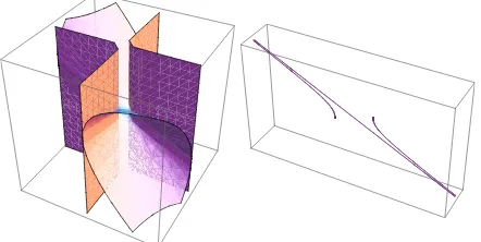
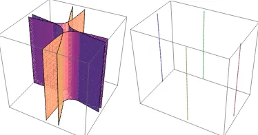
If we make a comparison with the 4th Runge-Kutta integrator, we obtain almost the same results, see Figures 5.1, 5.2 and 5.3, respectively, Figure 5.4. However Kahan’s integrator has the advantage to be easier implemented.
Fig. 5.1 The phase curves of the dynamics (1.1) for case (i)
Fig. 5.4 The phase curves of the dynamics (1.1) for case (ii) In this case Kahan’s integrator does not provide any relevant results.
References
[1] V. Arnold,Conditions for nonlinear stability of stationary plane curvilinear flows of an ideal fluid, Doklady 162, 5 (1965), 773-777.
[2] A. Aron, C. D˘an˘aias˘a, M. Puta,Quadratic and homogeneous Hamilton-Poisson systems on(so(3))∗
, Int. Journal of Geometric Methods in Modern Physics, 4, 7 (2007), 1173 - 1186.
[3] A. Aron, C. Pop, M. Puta, Quadratic and homogeneous Hamilton-Poisson sys-tems on (sl (2,R))* and Kahan’s integrator, In: (Eds.: D. Andrica, S. Moroianu), ”Contemporary Geometry and Topology and Related Topics”, Cluj-Napoca, Au-gust, 19-25, 2007, 63-72.
[4] B.H. Bermejo and V. Fair´en, Simple evaluation of Casimir invariants in finite dimensional Poisson systems, Phys. Lett. A 241 (1998), 148-154.
[5] L. Bianchi, Lezioni sulla teoria dei gruppi continui finite di trasformazioni, (1918), §198-199 (pp. 550-557). English translation by R.T. Jantzen, May 28, 1999.
[6] P. Birtea and M. Puta,Equivalence of energy methods in stability theory, Journ. of Math. Physics, 48, 4 (2007), 81-99.
[7] P.Birtea, M.Puta and R.M.Tudoran,Periodic orbits in the case of a zero eigen-value, C.R.Acad. Sci. Paris, 344, 12 (2007), 779-784.
[8] W. Kahan,Unconventional numerical methods for trajectory calculation, Unpub-lished Lecture Notes, 1993.
[9] L. Popescu,A note on Poisson-Lie algebroids (I), Balkan J. Geom. Appl. 14, 2 (2009), 79-89.
Authors’ addresses:
Anania Aron, Camelia Pop
”Politehnica” University of Timi¸soara, Department of Mathematics, Piat¸a Victoriei nr. 2, 300006-Timi¸soara, Romania.
E-mails: anania.girban@gmail.com , cariesanu@yahoo.com
Mircea Craioveanu