Is there a meaningful definition of
the value of a statistical life?
Per-Olov Johansson
∗Stockholm School of Economics, Box 6501, SE-113 83 Stockholm, Sweden
Received 6 January 2000; received in revised form 5 June 2000; accepted 6 September 2000
Abstract
A definition of the value of a statistical life is derived. This definition has a meaningful in-terpretation in terms of the monetary value of expected present value utility if consumption is age-independent. In all other cases, empirical estimates of the value of a statistical life are biased estimators of the monetary counterpart to expected present value utility. © 2001 Elsevier Science B.V. All rights reserved.
JEL classification:I10
Keywords:Value of a statistical life; Life expectancy; QALYs
1. Introduction
A central concept in health economics is the value of a statistical life. A common inter-pretation is as follows. Let us assume that the willingness-to-pay (WTP) for a programme saving two out of 10,000 lives is equal to $a. Then the value of a statistical life is equal to $a×10,000/2. This interpretation holds in a static or one-period setting. That is, it holds in a world, where people are either alive or dead during the entire time interval considered. In a truly intertemporal world, it is less obvious, how to define the value of a statistical life. However, if the reduction in the hazard rate lasts for 1 year, it might seem as if the above defi-nition still goes through. If the WTP for a 1-year-drop in the hazard rate equal to 2/10,000 is $a, it might seem reasonable to estimate the value of a statistical life to $a×10,000/2. If the duration of the drop in the hazard rate exceeds or falls short of 1 year, it seems as if one instead must base the definition on the change in life expectancy. To illustrate, let us assume that a programme extends the expected remaining length of life from 50 to 52 years. If the
∗Tel.:+46-8-736-92-82; fax:+46-8-30-21-15.
E-mail address:[email protected] (P.-O. Johansson).
associated WTP is $b, then a possible definition of the value of a statistical life seems to be $b×50/2.
This note derives a definition of the value of a statistical life for an intertemporal world. It is demonstrated that the above intuitive definitions are wrong. The correct definition must be based on the discounted values of remaining life expectancy and change in life expectancy, respectively. If consumption is constant over time, such a defined value of a statistical life is equal to the monetary counterpart to expected remaining present value utility. However, if consumption follows a non-constant path over the life cycle, the value of a statistical life overestimates or underestimates the monetary counterpart to expected remaining present value utility. Thus, unless consumption is age-independent, there seems to be no way to obtain an exact estimate of the monetary value of expected remaining present value utility.
2. The model
Let us consider anτ-year-old individual who consumes a single good.1 His instantaneous utility function at agetis denotedu[c(t)], wherec(t) is consumption at aget, witht ≥τ. The individual’s survivor function, which yields the probability of becoming at leastt-year-old, is denotedµ(t). 2 Conditional on having survived until ageτ, the considered individual’s expected remaining present value utility is defined as follows.
E(uτ)=
Z ∞
τ
u[c(t )]e−θ (t−τ )µ(t;τ )dt (1)
Z ∞
τ
u[c(t )]e−θ (t−τ )µ(t )dt
whereEis an expectations operator,µ(t;τ )=µ(t )/µ(τ )the survivor function, conditional on having survived until ageτ, andθ the marginal rate of time preference for simplicity assumed to be age-independent. The right-hand side expression in Eq. (1) yields the present value at ageτof instantaneous utility at agetmultiplied by the probability of surviving for at leasttperiods/years, beyond ageτ summed (integrated) over the entire time horizon.
The individual maximises his expected remaining present value utility, conditional on having survived until ageτ, subject to the dynamic budget constraint:
˙
k(t )=r k(t )+w(t )−c(t )−CV(t ); k(τ )=kτ (2)
wheret ≥ τ,k(t) denotes assets at aget,rthe interest rate for simplicity assumed to be constant across time,w(t) a fixed income/pension at aget, CV(t) denotes a payment for a change in the survival probability, as is further explained below, CV(t) is set equal to 0 for allthere, andkτa constant representing initial assets.
1The model is adapted from Johannesson et al. (1997) and most technical considerations, such as properties of subutility functions, are skipped here.
2The survivor function of the individual is defined asµ(t )=e−Rt
The expected present value Hamiltonian at timet, conditional on having survived to age
τ, for this problem is written as
H (t )=u[c(t )]e−θ (t−τ )µ(t;τ )+λ(t )k(t )˙ (3) whereλ(t) is a present value costate variable, yielding present values at ageτ.
Assume that the individual studied has solved the maximisation problem stated in Eqs. (1) and (2); see Johannesson et al. (1997) for details. His maximal expected remaining present value utility at ageτ, conditional on having survived to ageτ, is defined as follows.
Vτ(τ )=
Z ∞
τ
u[c∗(t )]e−θ (t−τ )µ(t;τ )dt (4)
whereVτ(τ) denotes the value function, i.e. the solution of the maximisation problem in
Eqs. (1) and (2), conditional on having survived until ageτ, and an asterisk denotes a value along the optimal path. Thus, the value function yields expected remaining present value utility for a utility-maximising individual agedτ years (and can be interpreted as the intertemporal counterpart to the atemporal indirect utility function). The reader is referred to Section 3 for further illustration of the meaning of a value function.
Let us now consider a decrease in the hazard rate. This decrease might last for a short period of time or for the rest of the individual’s life. It occurs/begins at ageτ +T, where
T ≥0. The associated change in expected remaining present value utility is equal to
dVτ(τ )=
Z ∞
τ+T
u[c∗(t )]e−θ (t−τ )dµ(t;τ ) (5)
where dµ(t;τ) refers to the timetchange in the conditional survivor function caused by the considered change in the hazard rate. The dynamic envelope theorem ensures that the effect of induced changes in the optimal consumption path vanishes from the expression.3 This explains the fact that Eq. (5), only contains the direct impact of the change in the hazard rate. The change in the hazard rate has a direct impact on the survivor function, as is reflected by dµin Eq. (5).
Let us now consider the WTP for the change in expected remaining present value utility in Eq. (5). For simplicity, let us assume that the individual makes a once-and-for-all payment “today”, i.e. at ageτ, in exchange for the decrease in the hazard rate occurring at ageτ+T
and lasting over a certain time interval. This payment is such that his expected present value utility remains unchanged, i.e.
Z ∞
τ+T
u[c∗(t )]e−θ (t−τ )dµ(t;τ )−λ∗(τ )dCV(τ )=0 (6)
where dCV(τ) denotes the individual’s WTP “today”, i.e. at ageτ, for the considered change in the hazard rate. The costate variableλ∗(τ) can be interpreted as the expected present value of the marginal utility of income at ageτ (evaluated along the optimal path as the asterisk indicates). Eq. (6) can be derived by differentiating the Hamiltonian function in Eq. (5) with respect to a change in the hazard rate, integrating fromτ and onwards, and employing the
dynamic envelope theorem. The reader is referred to Johannesson et al. (1997) for a detailed derivation.
In order to be able to compare the WTP for different programmes affecting the hazard rate in different ways, the value of a statistical life is often used. The question arises, how to define the value of a statistical life in an intertemporal world. A reasonable demand is that the concept should reflect expected remaining present value utility as defined by the value function in Eq. (4). Therefore, let us examine whether Eq. (6) can be rewritten in such a way that we obtain a definition of the value of a statistical life such that it reflects expected remaining present value utility.
In order to arrive at a definition of the value of a statistical life, let us assume that
c∗(t )=c∗for alltin Eq. (6), i.e. consumption is constant over time.4 Then, we can factor out the constantu(c∗) from the integral in Eq. (6) and the expression can be rewritten in the following way.
Note that the denominator in the right-hand side expression in Eq. (7) yields the expected number of discounted life years gained through the considered programme. Next, let us multiply through Eq. (7) by the expected number of remaining discounted life years, i.e.
Z ∞
τ
e−θ (t−τ )µ(t;τ )dt (8)
Then, Eq. (7) can be written as follows.
1
The left-hand side and middle expressions in Eq. (9) yield the considered individual’s expected remaining present value utility converted from units of utility to monetary units by division byλ∗(τ), i.e. the “marginal utility of income”. The right-hand side expression provides a measure of Vτ(τ)/λ∗(τ) that can be estimated. This measure is, here, called
the value of a statistical life, because it yields a monetary measure of expected remaining present value utility.
value of a statistical life. Eq. (9) holds independently of whether the drop in the hazard rate lasts for a “moment” or for the rest of the person’s life.
It is important to note that a correct definition of the value of a statistical life is based on discounted life years, not on life years. To illustrate, let us return to the example given in Section 1, where an individual was willing to pay $bin exchange for a programme that extends his expected remaining length of life from 50 to 52 years. It would be wrong to calculate the value of a statistical life as $b×50/2, since each (existing as well as gained) life year should be discounted. This can be explained as follows. Let us consider two programmes that both are expected to extend life by 2 years (from 50 to 52 years). The first programme reduces the hazard rate immediately, while the second programme reduces the hazard rate 10 years from now. Obviously, the WTP for the first programme is higher than the WTP for the second programme. Using the formula $b×50/2, one would, hence, end up with two different estimates of the value of a statistical life. The discounting procedure in Eq. (9) aims at correcting for the fact that a decrease in the hazard rate occurring in a distant future is less valued today than a drop occurring closer to the present.
Let us next assume that optimal consumption follows a non-constant path. In this case, it is impossible to factor out the instantaneous utility function and proceed in the way used in arriving at Eq. (9). Instead, we arrive at the following messy expression
Vτ(τ )
It should be noted that the left-hand side expression, i.e. the monetary value of expected remaining present value utility, differ from the middle and right-hand side expressions. Thus, the right-hand side expression, which we can estimate empirically, no longer provides an exact measure of the monetary value of the individual’s expected remaining present value utility, i.e. ofVτ(τ)/λ∗(τ). The problem is the fact that consumption varies over time, i.e.
we cannot factor out the instantaneous utility functionu[c∗(t)] from the first integral in the middle expression.6 Since utility varies over time, the instantaneous utility level obtained at a particular point in time must be “discounted” by the product of the utility discount factor and the survivor probability at that time. In other words, the individual’s expected remaining present value utility is dependent on the consumption pattern over the life cycle. For example, if consumption is increasing in age, then an extra unit of consumption will yield lower utility at an advanced age than at young age. The empirical estimate of the value of a statistical life, i.e. the right-hand side expression in Eq. (10), fails to recognise this fact. Thus, it seems impossible to provide an exact empirical estimate ofVτ(τ)/λ∗(τ), unless
we can reasonably assume that consumption is constant over time, i.e. is independent of the individual’s age. In other words, empirical estimates of the value of a statistical life are biased measures of the monetary value of expected remaining present value utility, in general. However, one would expect that the shorter period of time the drop in the hazard rate
lasts, the more reasonable is the “approximation” provided by the right-hand side expression in Eq. (10); see Section 3 for an illustration of this claim.
Finally, let us consider the question whether the WTP for quality-adjusted life years (QALYs) can be used to estimate the value of a statistical life. Bleichrodt and Quiggin (1999) show that under certain assumptions one can derive a tractable expression for the WTP for QALYs; under these assumptions cost-effectiveness analysis is consistent with cost–benefit analysis. In order to illustrate, let us assume that the instantaneous utility function is equal tou[c(t)]q[h(t)], whereq[h(t)] is the quality weight or utility of health h(t) at timet. Moreover, let us assume that optimal consumption and optimal health are both constant over time, i.e.c(t ) =candh(t ) = hfor allt; this assumption is used by Bleichrodt and Quiggin (1999) to establish the equivalence of cost-effectiveness analysis and cost–benefit analysis. Finally, let us consider a permanent marginal change in health (occurring at ageτ). Then the counterpart to Eq. (6) would read
qh(h)dh
Z ∞
τ
u(c)e−θ (t−τ )µ(t;τ )dt−λ(τ )dCV(τ )=0 (6′)
where a subscripthrefers to a partial derivative with respect toh. Multiplying through out byq(h)/λ(τ)qh(h)dhyields
whereVτ(τ) is the value function conditional on surviving until ageτ. The left-hand side
and middle expressions in Eq. (9′) yield a monetary measure of expected remaining present
value utility of a person agedτ years. The right-hand side expression yields the WTP for a marginal change in quality of life times actual quality of life.7Thus, the assumptions needed in establishing the equivalence of cost-effectiveness analysis and cost–benefit analysis, and derived by Bleichrodt and Quiggin (1999), are also needed in providing an exact and meaningful definition of the value of a statistical life.
3. A numerical illustration
In order to illustrate some of the theoretical results derived in Section 2, a simple numerical model is presented. The individual is assumed to solve the maximisation problem
Max
alltin the base case. For the sake of simplicity, a newly born individual is considered, i.e.
7If the change in health lasts over the interval (τ,T), the right-hand side expression in Eq. (9′) would read
dCV(τ )(q(h)R∞
t e−θ (t−τ )µ(t;τ )dt )/(qh(h)dh RT
τ e−θ (t−τ )µ(t;τ )dt ). Then dCV refers to the WTP for an
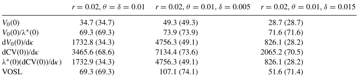
Table 1
Numerical estimations of the value of a statistical life (VOSL)a
r=0.02,θ=δ=0.01 r=0.02,θ=0.01,δ=0.005 r=0.02,θ=0.01,δ=0.015
V0(0) 34.7 (34.7) 49.3 (49.3) 28.7 (28.7)
V0(0)/λ∗(0) 69.3 (69.3) 73.9 (73.9) 71.6 (71.6) dV0(0)/dκ 1732.8 (34.3) 4756.3 (49.1) 826.1 (28.2) dCV(0))/dκ 3465.6 (68.6) 7134.4 (73.6) 2065.2 (70.5)
λ∗(0)(dCV(0))/dκ) 1732.9 (34.3) 4756.3 (49.1) 826.1 (28.2)
VOSL 69.3 (69.3) 107.1 (74.1) 51.6 (71.4)
aValues reported within parentheses refer to the case, whereε=1.
τ =0 in Eq. (11). Optimal consumption at timetis equal toc∗(t )=(θ+δ)k0e(r-θ-δ)t, wherek0denotes initial assets and any wage income is ignored; the reader is referred to Léonard and van Long (1992, pp. 290–292) for a detailed discussion of this model. Thus, consumption is increasing or decreasing over time ifr 6=θ+δ. The value function, see Eq. (4), is obtained by substitution ofc∗(t )=(θ+δ)k0e(r−θ−δ)tinto the right-hand side expression in Eq. (11). Solving the resulting expression one obtainsV0(0)=(θ+δ)−1[((r−
θ−δ)/(θ+δ))+ln(k0(θ+δ))], as is shown in detail in Léonard and van Long (1992).8 In the simulations, a change in the hazard rate is modelled as follows.9 We set dβ(t )=teκtdκ
fort∈[0, ε], and dβ(t )=εeκεdκfort ∈(ε,∞]. This approach is used because, it allows us to consider a change in the hazard rate lasting for an arbitrary number of periods. Two different cases,ε = 1 and 500, will be considered, and it is assumed thatκ =0. Initial assets, i.e.k0, are set equal to 100.
The results are reported in Table 1 (and Mathematica 4 was used for the numerical calculations). The infinitesimally small drop in the hazard rate κ lasts either “forever” (ε=500) or for 1 year (ε=1). The results relating to the 1-year decrease in the hazard rate are reported within parentheses in the table. Initial expected present value utility is denoted V0(0) and its monetary counterpart is denotedV0(0)/λ∗(0), where λ∗(0) is the costate variable (i.e. the marginal utility of income) at time zero.10 The change in expected present value utility caused by an infinitesimally small decrease in the hazard rate is denoted dV0(0)/dκ in the table,11 while the WTP for the considered decrease in the hazard rate is denoted dCV(0)/dκ (and in the column 2 case, whereδ = 0.01, this amount should be multiplied by a factor 0.001 in order to reflect a 10% drop in the hazard rate). Multiplying the WTP by the costate variableλ∗(0) yields an estimate of dV0(0)/dκ. The label VOSL in the table refers to the right-hand side expression in Eq. (9) (or Eq. (10)), i.e. to the value of a statistical life.
8However, the reader should replace the terminal condition (9.9c) in L´eonard and van Long (1992, p. 290), i.e. limt→∞k(t )=0, by the No-Ponzi game condition limt→∞k(t )e−rt=0, since we here consider an individual’s
maximisation problem (and, therefore, must respect his dynamic budget constraint). The No-Ponzi game condition prevents the individual from borrowing unlimited amounts. The utility discount rate used by L´eonard and van Long is interpreted as equal to the sum ofθandδin Eq. (11).
9The reader is referred to Johannesson et al. (1997) for details. 10It holds thatλ∗(t )=e−rt/((θ+δ)k
0)for the model under consideration. Moreover, it is easily verified that dV0(0)/dk0=1/((θ+δ)k0), i.e. is equal toλ∗(0).
11Since the drop in the hazard rate is evaluated atκ=0, the change in expected present value utility is simply equal to dV0(0)/dκ=
Rε
0ln[c∗(t )]e−θ te−δttdt+
R∞
Let us first consider the case where optimal consumption is constant over time. This case is reported in the second column of Table 1. Then the VOSL is equal to the monetary value of the individual’s expected present value utility, i.e.V0(0)/λ∗(0). This holds regardless of the length of the decrease in the hazard rate. However, if consumption is increasing over time, our approach would overestimateV0(0)/λ∗(0). This is shown in the third column of the table. The estimate of the VOSL does not capture the fact that the marginal utility of consumption is decreasing in age since consumption is increasing in age. As a consequence, the overestimation would be even more pronounced if the treatment/programme was un-dertaken at a future point in time. On the other hand, if consumption is decreasing in age, so that the marginal utility of consumption is increasing in age, the empirical VOSL esti-mate would underestiesti-mateV0(0)/λ∗(0). This is shown in the final column of the table. If consumption is non-constant over time, i.e. ifr 6=θ+δ, VOSL provides a more accurate estimate ofV0(0)/λ∗(0) if the reduction in the hazard rate lasts over a short time interval than if it lasts over a longer time interval. This can be seen by comparing the VOSL for
ε=1 and 500, respectively.
4. A concluding remark
This paper has provided a definition of the value of a statistical life that can be estimated empirically. However, such a measure is not necessarily a good indicator of the monetary value of expected present value utility. It works, if consumption is constant over the life cycle. If consumption is decreasing or increasing over time, the value of a statistical life (VOSL) becomes a poor indicator of the monetary value of expected present value utility. In particular, this is true if the change in the hazard rate used in calculating the VOSL lasts for a long period of time. One would expect that it is even more difficult to give empirical VOSL-measures a meaningful interpretation in a world where individuals value other things than consumption of private goods, say, their health, unless all involved values are constant over the entire life cycle.12
Acknowledgements
I am grateful to Magnus Johannesson for helpful comments as well as for calling my attention to the paper by Bleichrodt and Quiggin. I am also grateful for comments provided by two referees.
References
Aronsson, T., Johansson, P.-O., Löfgren, K.-G., 1994. Welfare measurement and the health environment. Annals of Operations Research 54, 203–215.
Bleichrodt, H., Quiggin, J., 1999. Life-cycle preferences over consumption and health: when is cost-effectiveness analysis equivalent to cost–benefit analysis? Journal of Health Economics 18, 681–708.
Johannesson, M., Johansson, P.-O., Löfgren, K.-G., 1997. On the value of changes in life expectancy: blips versus parametric changes. Journal of Risk and Uncertainty 15, 221–239.
Léonard, D., van Long, N., 1992. Optimal Control Theory and Static Optimization in Economics. Cambridge University Press, New York.