Full Terms & Conditions of access and use can be found at
http://www.tandfonline.com/action/journalInformation?journalCode=ubes20
Download by: [Universitas Maritim Raja Ali Haji] Date: 11 January 2016, At: 22:50
Journal of Business & Economic Statistics
ISSN: 0735-0015 (Print) 1537-2707 (Online) Journal homepage: http://www.tandfonline.com/loi/ubes20
Measuring Segregation When Units are Small: A
Parametric Approach
Roland Rathelot
To cite this article: Roland Rathelot (2012) Measuring Segregation When Units are Small: A Parametric Approach, Journal of Business & Economic Statistics, 30:4, 546-553, DOI: 10.1080/07350015.2012.707586
To link to this article: http://dx.doi.org/10.1080/07350015.2012.707586
View supplementary material
Accepted author version posted online: 11 Jul 2012.
Submit your article to this journal
Article views: 238
Measuring Segregation When Units are Small:
A Parametric Approach
Roland R
ATHELOTCREST, B ˆatiment MK2 Bureau 2020, Timbre J310, 15 Boulevard Gabriel P ´eri, 92245 Malakoff Cedex, France ([email protected])
This article considers the issue of measuring segregation in a population of units that contain few individuals (e.g., establishments, classrooms). When units are small, the usual segregation indices, which are based on sample proportions, are biased. We propose a parametric solution: the probability that an individual within a given unit belongs to the minority is assumed to be distributed as a mixture of Beta distributions. The model can be estimated and indices deduced. Simulations show that this new method performs well compared to existing ones, even in the case of misspecification. An application to residential segregation in France according to parents’ nationalities is then undertaken. This article has online supplementary materials.
KEY WORDS: Beta-binomial model; Dissimilarity index; Ethnic concentration; Mixture of Beta distributions.
1. INTRODUCTION
Standard segregation indices measure the distance between the distribution of a minority population across units and a counterfactual situation of evenness in which the proportion of minority individuals would be exactly the same in each unit. When units are small, past research has stressed that random-ness, a counterfactual situation in which the minority individuals are distributed randomly across units, would be a more sensi-ble benchmark than evenness (Cortese, Falk, and Cohen1976; Boisso et al.1994; Ransom2000). The discrepancy arises be-cause segregation indices use the observed proportionπaof the
minority group in unitato estimate the true unobserved proba-bilitypa that an individual of this unit belongs to the minority.
When units are small,πa is a noisy estimate ofpa and indices
are biased. This issue is of practical relevance: analyses that in-vestigate the distribution of employees across firms (Carrington and Troske1995; Kramarz, Lollivier, and Pel´e1996; Kremer and Maskin1996; Carrington and Troske1998b; Bayard et al. 1999; Hellerstein and Neumark2008), pupils across schools or classrooms (Allen, Burgess, and Windmeijer2009; S¨oderstr¨om and Uusitalo2010), or inhabitants across districts or buildings (Maurin2004) may be directly affected by this small-unit bias. Following Winship (1977), Carrington and Troske (1997)— hereafter CT—introduced an adjusted index. Their approach is the most frequently used in the applied literature (Carrington and Troske 1998a; Hellerstein and Neumark 2003, 2008; Persson and Sj¨ogren Lindquist2010; S¨oderstr¨om and Uusitalo 2010) and has been extended to account for the presence of covariates (Aslund and Skans 2009). Allen, Burgess, and Windmeijer (2009)—hereafter ABW—proposed to correct indices by a bootstrap procedure and provide simulations to show its performance. Both CT and ABW emphasized the issue of inference and proposed statistical tests of segregation.
In this article, an alternative method based on parametric assumptions is proposed to deal with the small-unit issue. First, a statistical framework is introduced: the probabilitypa
is assumed to be a random variable with distribution F. The
distribution of the number of minority individuals in unitais then a binomial with parameterspaand the unit size. To compute
a distance to randomness, one would like to usepainstead of the
empirical proportionsπato compute the segregation index. The
index based on the unobserved probabilitiespais the quantity of
interest of this analysis. The main contribution of this article is to propose a simple parametric approach to estimate this index of interest:Fis assumed to be a mixture of Beta distributions. Under this assumption, the parameters of the distribution and therefore the quantity of interest can be estimated. The model is an extension of the Beta-binomial model and offers an apprecia-ble trade-off between flexibility and parsimony. Both bootstrap and the delta method may be used to provide for inference.
I compare to what extent the existing methods estimate the quantity of interest of this article. In expectation, the CT-adjusted index is shown to be below the quantity of interest when applied to the dissimilarity index, except when the underlying distribu-tion is discrete with three masspoints—on 0, 1, and the mean of the distribution. Simulations are also run to compare the meth-ods proposed by CT and ABW to the one that I propose here, for the dissimilarity, the Gini, and the Theil indices. These simula-tions show that the correction method relying on the estimation of a Beta mixture performs well in various cases, including those in which the parametric model is misspecified.
Finally, the Beta-mixture correction method is applied to mea-sure the residential segregation of first- and second-generation migrants, according to their country of origin, in France. This case illustrates well the small-unit issue, as the only available data is a survey in which the number of individuals by unit is equal to 30 on average, while the minority groups represent between 0.2% and 6% of the total population.
The next section details the statistical framework and presents the existing methods that attempt to deal with the issue. Section3
© 2012American Statistical Association Journal of Business & Economic Statistics
October 2012, Vol. 30, No. 4 DOI:10.1080/07350015.2012.707586
546
Rathelot: Measuring Segregation When Units are Small 547
presents the new method introduced in this article. Section4 shows how the proposed approach performs on simulated data, compared to existing methods. Section5presents an application to ethnic residential segregation in the French case.
2. THE PROBLEM AND ITS EXISTING SOLUTIONS
Concentration indices are useful tools to capture the uneven-ness of the distribution of different groups in different units (Duncan and Duncan 1955; Cortese, Falk, and Cohen 1976, 1978; James and Taeuber 1985; Massey and Denton 1988; Hutchens2004).Evennessrefers to actual equality across units: if firms have 10 employees and if there are as many men as women in the working population, evenness occurs if there are exactly five men and five women in each firm.Random alloca-tionimplies that theprobabilitiesfor a given individual to be a woman (or a man) are equal in all firms, even if strict equal-ity in actualproportionsis not reached. This article presents a measure from randomness rather than evenness, as the former benchmark is interesting to many practitioners.
2.1 Statistical Framework
The population is assumed to be split into two groups, a mi-nority group and the rest of the population, and to be distributed across Aunits, a=1, . . . , A. In practice, groups may be de-fined according to gender, nationality, ethnicity, or social status, while units may be businesses, schools, or neighborhoods. In the present analysis, the number of individuals in unita, denoted as Ma, is drawn from a given, unknown distribution. In the whole
analysis,Ais assumed to be large, whileMa is assumed to be
small.
Letpa denote the probability for an individual of unita to
be a member of the minority group. The random variablespa,
that take values in [0,1], are assumed iid in distributionF. The numberNaof individuals in unitathat belong to the minority is
observed and distributed as a Binomial(Ma, pa). WhileNaand
Maare perfectly observed,pais not. The observed sample
pro-portionπa =Na/Maof the minority group in unitais usually
used to estimatepa. If the numberMa of individuals in unita
goes to infinity,πais a consistent estimator ofpa; furthermore,
E[πa|pa]=pa, so that it is also an unbiased estimator.
2.2 Evenness, Randomness, and the Index of Interest
Segregation indices measuring distance from evenness can be defined as functions of a vector of proportions{πa}{a=1,...,A}: let ˜I denote these “direct indices.” Let ¯p=
aNa/aMa
denote the sample mean; note that ¯p is an unbiased estima-tor ofE(p) whatever the unit size. Three indices are used in this article—the Gini index, the dissimilarity (or Duncan) in-dex, and the Theil index (see, for instance, Massey and Denton 1988, for a review of the properties of these indices)—but the analysis can be generalized to any concentration index. Defining wa=Ma/a′Ma′ as the weight of unita in the sample, the direct versions of these indices, in the two-group case, can be
expressed as
The random-allocation valueI∗is defined as the expectation of ˜I, conditional on all units being assigned the same probability pa =µ. When the probabilities of all units are equal to µ(a
distribution denoted as Dµ), the unevenness is entirely due to random allocation and E( ˜I)=I∗. To measure the distance to randomness, the index of interest should not be computed with the proportionsπabut with the unobserved probabilitiespa. The
expectation of the index based on the probabilitiespa depends
on the distributionFand is therefore denoted asI(F). For the Gini, the dissimilarity, and the Theil indices, the expressions as functionals ofFare the following (see the online Appendix for details):
direct indices ˜I biased estimates ofI(F). The expected small-unit bias is defined as the difference betweenE( ˜I) andI(F).
How large is the bias in practice? Cortese, Falk, and Cohen (1976) and CT ran simulations that showed how relevant the issue is; I reproduce these simulations for the dissimilarity index (the setting and the results are presented in the online Appendix). Two conclusions can be drawn from this exercise. First, the magnitude of the bias, around 0.5 for units of 15 people and a minority proportion of 5%, makes it an issue one cannot neglect. Second, the bias decreases with the unit size and with the total share of the minority group.
2.3 Existing Methods
CT propose a measure of the departure from randomness, based on the Euclidean distance between ˜Iand ˆI∗, a simulation-based estimate ofI∗:
As CT do not make any assumption about the data-generating process (dgp) of (Na, Ma), there is no reason whyICT would
converge toI(F). Still,E(ICT) happens to coincide withI(F) in
some cases. When the distribution ofpaisDµ,E(ICT)=I(F)=
0. When, conversely,pa =1 in some units whilepa =0 in all
the others (a distribution denoted as D0,1(µ), whereµ is the
weight on value 1), ˜I =ICT=1=I(F) for all samples. For
every concave mixture between the discrete distributions Dµ andD0,1(µ) (denoted asD0,µ,1(w), where wis the weight on the distributionDµ), it can be proved thatE(ICT)=I(F).
More precisely, three conclusions can be established for the Theil and the dissimilarity indices (see the online Appendix for a formal proof). First, when the true distribution is one of the familyD0,µ,1(w), the CT adjustment leads toI(F):E(ICT)= I(F). For the dissimilarity index, this implication turns out to be an equivalence. For every other distribution, continuous or discrete, the CT adjustment leads, on average, to a lower value thanD(F):E(DCT)< D(F). Finally, for the Theil index, there
is no such property. The difference betweenHCTandH(F) may
be positive or negative, depending on the distribution.
ABW proposed to use bootstrap techniques to adjust the index for the presence of a potential bias. Given the unit sizeMaand
the observed proportionsπa, they simulateBsamples, drawing
Na(b),b=1, . . . , B. For each simulated sample b, an index
˜
I(b) is computed. The corrected index they proposed is then
IABW =. 2 ˜I−
unit bias and that adding it to ˜I provides an estimator for the unbiased estimator. This strategy succeeds in reducing the order of the bias fromO(1/M) toO(1/M3/2) or evenO(1/M2).
Section4proposes simulations to assess whether the adjusted indices proposed by CT and ABW fall close to or far fromI(F).
3. A PARAMETRIC METHOD
Unlike existing methods, this article proposes a correction method based on a parametric assumption: pa is distributed
as a mixture of Beta distributions. Since its formalization by Skellam (1948), the Beta-binomial model has been used in various fields (e.g., Lee and Sabavala 1987; Cox and Katz 1999; Cogley and Sargent 2009) and has three main virtues. First, the Beta distribution is the conjugate prior of the binomial distribution (Greenwood 1913). Second, the model is parsimonious: 3c−1 parameters are enough to describe a c-component mixture of Beta distributions. Third, Beta distributions encompass many different cases.
One may object that a parametric approach may lead to in-valid results when the model is misspecified. Two arguments can be used to support this approach. First, Diaconis and Ylvisaker (1985, Theorem 1) pointed out thatc-component mixtures of Beta distributions are dense in the space of the continuous dis-tributions on the unit interval. Second, in the present case, the results of simulations with various dgp show that, using mix-tures with at most two components, the segregation indices cor-responding to both continuous and discrete distributions are accurately proxied by the mixtures (see Section4).
LetB(., .) denote the Beta function,v= {αj, βj, λj}j∈{1,...,c} the vector of parameters with
jλj =1. The pdf of the rvpa,
distributed as ac-component mixture of Beta distributions, is
fv(p)
The probability that n individuals out of m belong to the minority group can be written, after some algebra, as
P(Na=n|Ma =m)=
Conditional on the unit sizeMa, the probability expressed
in Equation (4) is the likelihood that a unitawill contain Na
persons from the minority population out of a total ofMa. LetAnm
denote the number of units of sizemwithnminority individuals; the log-likelihood may be written as
ℓm(v)=
Assuming that the same model holds for a set of units of size belonging to M= {m1, . . . , mr}, maximizing ℓM(v)=
m∈Mℓm(v) with respect tov provides the estimators ˆv(M).
In other words, instead of stratifying the sample by unit size, units of different sizes can be pooled in the same estimation. The setMshould be chosen by the practitioner, depending on the situation, from singleton sets to the entire support of the distribution of the unit size.
Once the parameters of the distribution are known, indices could be retrieved by simulations. However, in the case of this model, explicit expressions of the indices can be derived, to save computational time. The Gini, the dissimilarity, and the Theil indices admit the following expressions, as functions of the vector of parametersv(see the online Appendix for details):
G(v)=1− 2
Rathelot: Measuring Segregation When Units are Small 549
involves an integral that must be approximated by numerical methods.
Two methods may be used to provide inference on the in-dices based on the estimated values ˆv of the parameters. The delta method is easy to apply in this context as it only involves an estimate of the variance matrix of ˆvand of the derivative of the index with respect tov, evaluated at ˆv. The former is com-puted using the Hessian matrix, evaluated at ˆv, and the latter can be computed either analytically starting from Equations (6) to (8) or numerically, at little computational cost. The bootstrap, performed at the level of the units, can also be used. Both meth-ods provide very similar results in the simulations exercise and in the application; for the sake of readability, only the results of the delta method are reported.
Finally, how should the number of components of the mixture model be chosen? Given the estimation of the model forc−1 andccomponents, a likelihood-ratio test can be used iteratively to test whether the likelihood improvement is worth spending three additional degrees of freedom and which model should be preferred. Other methods of choosingccould also be used.
4. SIMULATIONS
As practitioners do not know a priori the distribution ofpa,
they expect bias-adjusting methods to work on the largest possi-ble spectrum. In this section, simulations using several continu-ous and discrete distributions are run to assess the performance of the method presented in this article, and to compare it to the solutions presented in CT and ABW. The unit size is fixed to 10 (in the online Appendix, simulations with a unit size of five are also presented). For each unit size and each distribution, 100 draws in 1000 units are made. Firstpais drawn iid in the given
distribution. Then,Nais drawn from a binomial with parameters
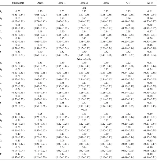
Ma, pa.Table 1displays the average values of the estimates, as
well as 95% confidence intervals.Table 2displays (100 times) their mean-squared errors (MSE), computed as the mean of the squared differences between the estimate and the value of the index based on probabilitiespa. Each panel of the tables is
ded-icated to a given index; the distributions of the dgp are in rows and the methods in columns.
In both tables, the first column presents the result for the direct estimates, computed with proportionsπa. Columns 2–4 show
the values obtained with the Beta-parametric method, assuming either a simple Beta model (column 2) or a mixture of two Beta distributions (column 3). In the fourth column, the best model (between Beta-1 and Beta-2) is chosen according to the result of a LR test, using a threshold of 0.05 for thep-value. In columns 5 and 6, the values relating to indices adjusted using CT and ABW methods are reported. InTable 1, the unfeasible estimate is also reported, to make comparisons easier.
Seven dgps of expectation 0.1 are tested. For B1, the dgp
is a Beta distribution of parameters (1, 9). ForB2, the dgp is
a mixture of two Beta distributions of parameters (1, 9) and (0.1, 0.9) with weights (0.7, 0.3). ForD1, the dgp is a discrete
distribution of support set (0, 0.1, 1) with associated weights (0.45, 0.5, 0.05). ForD2, the dgp is a discrete distribution of
support set (0.05, 0.1, 0.5) with associated weights (0.45, 0.5, 0.05). ForD3, the dgp is a discrete distribution of support set (0,
0.05, 0.1, 0.15, 0.2) with associated weights (0.2, 0.2, 0.2, 0.2, 0.2). ForN, the dgp is a truncated normal distribution of mean
0.1 and standard deviation 0.05. ForW, the dgp is a truncated Weibull distribution of parameters 0.1 and 1.1. Note that in all but the first two dgp, the Beta-binomial model is misspecified.
Consistently with earlier results, direct indices are found to suffer from large biases. Despite their imperfections, adjusting methods improve on the direct estimates in most cases. The comparison of the last five columns underlines the advantages and drawbacks of each method. As established in Section 2, the CT-adjusted dissimilarity index is always lower thanD(F), except when the true distribution is aD0,.1,1; interestingly, this seems to be also true for the Gini index. In many cases, for the Gini and the dissimilarity indices, the differences between the CT-adjusted indices andI(F) are of large magnitude, for example, 0.07 versus 0.21 with a truncated normal. Conversely, the CT adjustment almost coincides with I(F) for the Theil index. The indices corrected by the ABW method are upward biased in most cases. Their method performs better when the unfeasible index is high and when the distribution is continuous. For the Theil index, the ABW method is relatively less efficient than the other methods.
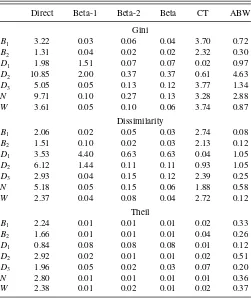
The Beta-1 correction, based on the assumption of a Beta distribution, is obviously at its best when the data are drawn from a Beta distribution. If the Normal, the Weibull, and even the discrete distribution with 5 support points are also satisfactorily dealt with, the discrete distributions with 3 support points lead to substantially higher MSE for the Gini and the dissimilarity indices. The Beta-2 correction improves on Beta-1 in the latter cases. The largest MSE (0.0063) of this method is obtained for the dissimilarity index with theD0,.1,1distribution, a value of the same magnitude as the MSEs experienced by the other methods in many cases. The Beta correction lies between Beta-1 and Beta-2: it allows flexibility when necessary while avoiding systematically overparameterizing the model.
Table 3sums up the results of the simulations. For each dgp and index, the table reports the method that leads to the estimator with the lowest MSE. When another method leads to a MSE lower than 0.001, it is reported in the second position. A rapid glance at the table shows that the Beta-mixture method is the one that gives, in most cases, the closest estimates toI(F). The only case in which the parametric method does not score best is the dissimilarity index with the discrete distributionsD0,.1,1.
5. APPLICATION
This section provides a first attempt to measure ethnic residen-tial segregation in France. As it is forbidden by law to collect race or ethnicity variables in France, the usual way to proxy ethnicity is to use parents’ nationality at birth (see, e.g., Meurs, Pailh´e, and Simon2006; Aeberhardt et al.2010). Unfortunately, while Censuses provide many variables (social and labor situa-tions, education, etc.) at the scale of the neighborhood, parents’ nationalities remain absent from this file, for legal reasons. The largest dataset in which parents’ nationalities are observed, since 2005, is the Labor Force Survey (LFS).
The sample design of the LFS defines ad hoc neighbor-hoods. Households are selected through a three-fold geographi-cal cluster sampling. The smallest clusters are thesampling units
(named “aires”) and have, on average, 20 contiguous house-holds. Households of a given sampling unit enter and leave the sample on the same quarter. The LFS dataset provides, for each
Table 1. Simulations: estimates with units of 10 individuals
Unfeasible Direct Beta-1 Beta-2 Beta CT ABW
Gini
B1 0.53 0.70 0.53 0.52 0.52 0.33 0.61
(0.51–0.54) (0.68–0.72) (0.48–0.56) (0.47–0.56) (0.48–0.56) (0.29–0.38) (0.58–0.64)
B2 0.69 0.80 0.71 0.69 0.69 0.54 0.74
(0.67–0.71) (0.78–0.82) (0.67–0.74) (0.66–0.73) (0.66–0.73) (0.49–0.59) (0.72–0.77)
D1 0.75 0.89 0.87 0.77 0.77 0.75 0.85
(0.71–0.78) (0.87–0.91) (0.84–0.89) (0.72–0.81) (0.72–0.81) (0.70–0.80) (0.82–0.87)
D2 0.36 0.69 0.50 0.34 0.34 0.28 0.57
(0.33–0.39) (0.66–0.71) (0.45–0.54) (0.25–0.46) (0.25–0.46) (0.23–0.34) (0.54–0.61)
D3 0.44 0.67 0.45 0.43 0.43 0.25 0.56
(0.42–0.46) (0.65–0.70) (0.39–0.49) (0.38–0.50) (0.38–0.50) (0.20–0.29) (0.53–0.60)
N 0.29 0.60 0.28 0.26 0.28 0.11 0.46
(0.28–0.30) (0.58–0.62) (0.22–0.34) (0.17–0.33) (0.21–0.34) (0.06–0.16) (0.43–0.49)
W 0.51 0.70 0.52 0.50 0.52 0.32 0.61
(0.50–0.53) (0.68–0.73) (0.47–0.56) (0.45–0.56) (0.47–0.56) (0.27–0.37) (0.58–0.64) Dissimilarity
B1 0.39 0.53 0.39 0.39 0.39 0.22 0.41
(0.37–0.40) (0.50–0.55) (0.35–0.42) (0.34–0.43) (0.35–0.42) (0.19–0.26) (0.37–0.44)
B2 0.51 0.64 0.54 0.52 0.52 0.37 0.54
(0.49–0.53) (0.61–0.66) (0.51–0.58) (0.49–0.55) (0.49–0.56) (0.34–0.42) (0.51–0.58)
D1 0.51 0.70 0.72 0.59 0.59 0.50 0.61
(0.47–0.56) (0.67–0.72) (0.69–0.75) (0.54–0.63) (0.54–0.63) (0.45–0.54) (0.57–0.65)
D2 0.25 0.49 0.36 0.27 0.27 0.15 0.35
(0.23–0.28) (0.47–0.52) (0.33–0.40) (0.21–0.33) (0.21–0.33) (0.12–0.19) (0.31–0.39)
D3 0.34 0.51 0.32 0.36 0.35 0.18 0.38
(0.32–0.35) (0.49–0.54) (0.28–0.36) (0.28–0.41) (0.28–0.41) (0.14–0.22) (0.35–0.42)
N 0.21 0.43 0.20 0.20 0.20 0.07 0.28
(0.20–0.22) (0.42–0.46) (0.16–0.24) (0.13–0.27) (0.14–0.25) (0.03–0.11) (0.25–0.32)
W 0.38 0.53 0.38 0.37 0.38 0.21 0.41
(0.36–0.39) (0.51–0.56) (0.34–0.42) (0.31–0.43) (0.34–0.42) (0.18–0.25) (0.37–0.45) Theil
B1 0.13 0.28 0.13 0.13 0.13 0.12 0.19
(0.12–0.14) (0.26–0.30) (0.11–0.15) (0.11–0.15) (0.11–0.15) (0.10–0.14) (0.17–0.21)
B2 0.26 0.38 0.25 0.25 0.25 0.24 0.31
(0.23–0.29) (0.36–0.41) (0.22–0.29) (0.22–0.29) (0.22–0.29) (0.20–0.28) (0.27–0.34)
D1 0.50 0.59 0.47 0.47 0.47 0.50 0.53
(0.46–0.54) (0.55–0.63) (0.43–0.52) (0.42–0.52) (0.42–0.52) (0.45–0.55) (0.49–0.58)
D2 0.10 0.27 0.11 0.10 0.10 0.11 0.17
(0.09–0.12) (0.26–0.29) (0.09–0.14) (0.08–0.13) (0.08–0.13) (0.09–0.14) (0.15–0.20)
D3 0.11 0.25 0.09 0.11 0.10 0.08 0.15
(0.10–0.12) (0.24–0.27) (0.07–0.11) (0.09–0.13) (0.07–0.13) (0.06–0.10) (0.13–0.17)
N 0.04 0.21 0.04 0.04 0.04 0.04 0.10
(0.04–0.04) (0.19–0.22) (0.02–0.05) (0.02–0.06) (0.02–0.05) (0.02–0.05) (0.08–0.12)
W 0.12 0.28 0.12 0.12 0.12 0.12 0.18
(0.12–0.13) (0.26–0.30) (0.10–0.15) (0.10–0.15) (0.10–0.15) (0.09–0.14) (0.16–0.21)
NOTE: For each distribution, simulations are based on 100 draws of samples of 1000 areal units, each consisting of 10 individuals. 95% confidence interval are showed in parentheses. ForB1, the dgp is a Beta distribution of parameters (1, 9). ForB2, the dgp is a mixture of 2 Beta distribution of parameters (1, 9) and (0.1, 0.9) with weights (0.7, 0.3). ForD1, the dgp is
a discrete distribution of support set (0, 0.1, 1) with associated weights (0.45, 0.5, 0.05). ForD2, the dgp is a discrete distribution of support set (0.05, 0.1, 0.5) with associated weights
(0.45, 0.5, 0.05). ForD3, the dgp is a discrete distribution of support set (0, 0.05, 0.1, 0.15, 0.2) with associated weights (0.2, 0.2, 0.2, 0.2, 0.2). ForN, the dgp is a truncated normal
distribution of mean 0.1 and standard deviation 0.05. ForW, the dgp is a truncated Weibull distribution of parameters 0.1 and 1.1. Source: Simulations by the author.
individual, an encrypted version of the ID of their sampling unit: the researcher knows whether two individuals live in the same unit, but not the unit’s location.
The mean size of a sampling unit is 30; the median is 31; 25% of the sampling units are smaller than 20 and 91% smaller than 50 (see the online Appendix for the complete distribution). Maurin (2004) used the LFS to obtain concentration measures
of social status and ethnicity but, because of the small-unit is-sue, did not use the usual indices. Small-unit issues are likely to be aggravated by the relative scarcity of ethnic minorities com-pared to French individuals of French origin. A complementary analysis conducted at an aggregated level shows that small-unit issues are not negligible, even with unit sizes around 100, when the minority share is below 5% (see Rathelot2011, for details).
Rathelot: Measuring Segregation When Units are Small 551
Table 2. Simulations: mean-squared errors (×100) with units of 10 individuals
Direct Beta-1 Beta-2 Beta CT ABW
Gini
B1 3.22 0.03 0.06 0.04 3.70 0.72
B2 1.31 0.04 0.02 0.02 2.32 0.30
D1 1.98 1.51 0.07 0.07 0.02 0.97
D2 10.85 2.00 0.37 0.37 0.61 4.63
D3 5.05 0.05 0.13 0.12 3.77 1.34
N 9.71 0.10 0.27 0.13 3.28 2.88 W 3.61 0.05 0.10 0.06 3.74 0.87
Dissimilarity
B1 2.06 0.02 0.05 0.03 2.74 0.08
B2 1.51 0.10 0.02 0.03 2.13 0.12
D1 3.53 4.40 0.63 0.63 0.04 1.05
D2 6.12 1.44 0.11 0.11 0.93 1.05
D3 2.93 0.04 0.15 0.12 2.39 0.25
N 5.18 0.05 0.15 0.06 1.88 0.58 W 2.37 0.04 0.08 0.04 2.72 0.12
Theil
B1 2.24 0.01 0.01 0.01 0.02 0.33
B2 1.66 0.01 0.01 0.01 0.04 0.26
D1 0.84 0.08 0.08 0.08 0.01 0.12
D2 2.92 0.02 0.01 0.01 0.02 0.51
D3 1.96 0.05 0.02 0.03 0.07 0.20
N 2.80 0.01 0.01 0.01 0.01 0.36 W 2.38 0.01 0.02 0.01 0.02 0.37
NOTE: For each distribution, simulations are based on 100 draws of samples of 1000 areal units, each consisting of 10 individuals. For the sake of clarity, values in the table are actually 100 times the MSE. ForB1, the dgp is a Beta distribution of parameters (1, 9).
ForB2, the dgp is a mixture of 2 Beta distribution of parameters (1, 9) and (0.1, 0.9) with
weights (0.7, 0.3). ForD1, the dgp is a discrete distribution of support set (0, 0.1, 1) with
associated weights (0.45, 0.5, 0.05). ForD2, the dgp is a discrete distribution of support
set (0.05, 0.1, 0.5) with associated weights (0.45, 0.5, 0.05). ForD3, the dgp is a discrete
distribution of support set (0, 0.05, 0.1, 0.15, 0.2) with associated weights (0.2, 0.2, 0.2, 0.2, 0.2). ForN, the dgp is a truncated normal distribution of mean 0.1 and standard deviation 0.05. ForW, the dgp is a truncated Weibull distribution of parameters 0.1 and 1.1. Source: Simulations by the author.
The Beta-binomial adjusting method is applied to the LFS from 2005 to 2008 for the shares of ethnic minorities within sampling units, on three populations. The first population are all individuals with foreign parents, whether they are themselves immigrants or not. The second population (“immigrants”) is a subsample of the first one, with only the immigrants who arrived in France after the age of 3. The third population (“French-born”) is the complement of the second population: only those
Table 3. Simulations: which method should be preferred in which case
Gini Dissimilarity Theil
B1 Beta Beta, ABW Beta, CT
B2 Beta Beta Beta, CT
D1 CT, Beta CT CT, Beta
D2 Beta Beta Beta, CT
D3 Beta Beta Beta, CT
N Beta Beta Beta, CT
W Beta Beta Beta, CT
NOTE: This table is a summary ofTable 1. For each distribution and each index, the least-biased method is reported. If other methods provide estimates with a 100×MSE lower that 0.10, they appear in second (and third if necessary) positions. ForB1, the dgp is a
Beta distribution of parameters (1, 9). ForB2, the dgp is a mixture of 2 Beta distribution
of parameters (1, 9) and (0.1, 0.9) with weights (0.3, 0.7). ForD1, the dgp is a discrete
distribution of support set (0, 0.1, 1) with associated weights (0.45, 0.5, 0.05). ForD2,
the dgp is a discrete distribution of support set (0.05, 0.1, 0.5) with associated weights (0.45, 0.5, 0.05). ForD3, the dgp is a discrete distribution of support set (0, 0.05, 0.1, 0.15,
0.2) with associated weights (0.2, 0.2, 0.2, 0.2, 0.2). ForN, the dgp is a truncated normal distribution of mean 0.1 and standard deviation 0.05. ForW, the dgp is a truncated Weibull distribution of parameters 0.1 and 1.1.
Source: Simulations by the author.
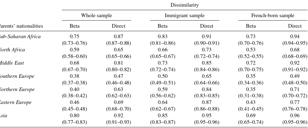
individuals born in France or who arrived before the age of 3. Minority groups (“Sub-Saharan Africa,” “North Africa,” “Mid-dle East,” “Southern Europe,” “Northern Europe,” “Eastern Europe,” and “Asia”) are defined according to parents’ national-ities (at least one of them). Individuals from “Northern Europe,” “Eastern Europe,” and “Asia” are required to have at least one parent of the corresponding nationality. For each minority group, the sample size and the proportion in the whole popula-tion are reported inTable 4. Individuals with parents from North Africa and Southern Europe are by far the most common. To-gether, they represent more than 10% of the population living in France; half of them are immigrant and half were born in France. The results for the dissimilarity index are reported in Table 5 (see the online Appendix for the Gini and the Theil). Columns 1 and 2 present the results on the whole population, columns 3 and 4 on the immigrant sample, and columns 5 and 6 on the French-born sample. For each population, the first column presents the index computed with the Beta method and the second one the index computed directly using sample proportions. As noted above, direct indices differ dramatically from the Beta-adjusted ones.
This application provides an interesting example of how use-ful accounting for the small-unit issue is. For all ethnic groups
Table 4. Sample size and proportions of the main ethnic minorities in France
Whole sample Immigrant sample French-born sample
Parents’ nationalities Sample size Proportion Sample size Proportion Sample size Proportion
Sub-Saharan Africa 2474 0.8% 1765 0.6% 709 0.2%
North Africa 14826 4.8% 8528 2.7% 6298 2.0%
Middle East 4462 1.4% 3302 1.1% 1160 0.4%
Southern Europe 18335 5.9% 6841 2.2% 11494 3.7%
Northern Europe 5970 1.9% 2388 0.8% 3582 1.2%
Eastern Europe 4659 1.5% 1917 0.6% 2742 0.9%
Asia 1173 0.4% 692 0.2% 481 0.2%
NOTE: Columns 1, 3, and 5 report sample size; columns 2, 4, and 6 report proportions with respect to the total sample (representative of individuals of more than 16 living in France). Source: Labor Force Survey 2005–2008 (Insee).
Table 5. Segregation indices, by parents’ nationalities
Dissimilarity
Whole sample Immigrant sample French-born sample
Parents’ nationalities Beta Direct Beta Direct Beta Direct
Sub-Saharan Africa 0.75 0.87 0.83 0.91 0.73 0.94
(0.73–0.76) (0.87–0.88) (0.81–0.86) (0.90–0.91) (0.70–0.76) (0.94–0.95)
North Africa 0.59 0.65 0.66 0.73 0.53 0.68
(0.58–0.60) (0.65–0.66) (0.65–0.67) (0.72–0.74) (0.52–0.55) (0.68–0.69)
Middle East 0.68 0.81 0.73 0.85 0.72 0.92
(0.67–0.70) (0.80–0.82) (0.72–0.74) (0.84–0.86) (0.70–0.75) (0.91–0.92)
Southern Europe 0.38 0.47 0.50 0.65 0.35 0.49
(0.37–0.38) (0.46–0.48) (0.49–0.51) (0.64–0.66) (0.34–0.36) (0.48–0.50)
Northern Europe 0.40 0.63 0.59 0.84 0.35 0.71
(0.38–0.42) (0.62–0.63) (0.56–0.62) (0.83–0.85) (0.31–0.38) (0.70–0.72)
Eastern Europe 0.46 0.69 0.64 0.87 0.43 0.77
(0.45–0.48) (0.68–0.70) (0.62–0.67) (0.86–0.88) (0.41–0.45) (0.76–0.78)
Asia 0.80 0.92 0.85 0.95 0.69 0.96
(0.77–0.83) (0.91–0.93) (0.83–0.87) (0.95–0.96) (0.65–0.74) (0.95–0.96)
NOTE: Segregation is measured at the level of the sampling unit of the LFS. The first three columns present the indices computed after the estimation of the Beta model. The last three columns present the indices directly computed with the observed proportions. Confidence intervals at the level of 5% are displayed in parentheses.
Source: Labor Force Survey 2005–2008 (Insee).
but Europeans, the proportion of immigrants is higher than the proportion of French-born individuals. In the case of Africa and Asia, for instance, the direct index that measures the distance to evenness is higher in the French-born group than in the im-migrant one while the Beta index gives the opposite ranking. Accounting for small units also enables one to compare ethnic groups with each other, even when some groups are more fre-quent than others. According to direct indices, immigrants from Northern Europe are more segregated than those from North Africa; the Beta indices lead to the opposite result.
Finally, two groups may be distinguished in the whole sample: those with European parents are the least segregated, while those with African or Middle Eastern parents are the most segregated. For the French-born group, this ranking is not much different; the values are smaller but are more contrasted. The least segregated individuals are those with parents from Southern and Northern Europe, while individuals with parents from Asia, the Middle East, and Sub-Saharan Africa are the most segregated group. Focusing on immigrants, indices are substantially higher and closer to each other and the ranking changes marginally. Immigrants from Southern Europe are the least segregated while those from Sub-Saharan Africa and Asia are the most segregated.
6. CONCLUSION
When units (neighborhoods, businesses, classrooms) have few observations, the standard indices, which measure a dis-tance to evenness, are not relevant: the desirable benchmark is randomness. The small-unit issue occurs because standard in-dices use minority shares to proxy the true probabilities that an individual of the unit belongs to the minority group. This arti-cle presents a statistical framework that provides a natural way to define the index of interest: the unfeasible one that would be based on these true unobserved probabilities instead of
esti-mated shares. A new method is proposed to estimate this index of interest. Assuming that the distribution of the probabilities is a mixture of Beta distributions, the parameters of the distribution can be estimated, and segregation indices deduced.
This new method is compared to the two main existing meth-ods, introduced by Carrington and Troske (1997) and Allen, Burgess, and Windmeijer (2009), using simulations. In most cases, which are not restricted to data-generating processes distributed as Beta mixtures, the new method is shown to fall closer to the quantity of interest. One should stress, however, that Carrington and Troske (1997) did not claim to estimate the same quantity of interest, so that the differences between their adjusted index and our quantity of interest cannot be interpreted as bias. An application provides the first available figures about ethnic residential segregation in France, using the LFS and its unique sampling scheme to define neighborhoods. French individuals whose parents are immigrants experience levels of residential segregation that vary much across countries of origin. Individuals with parents from Sub-Saharan Africa, the Middle East, and North Africa experience higher levels of residential concentration than those with parents coming from Europe.
Several extensions of the present method would be useful for practitioners. First, when covariatesXare observed for individ-uals (and units), the practitioner might wish to measure to what extent segregation can be attributed by differences in covariates between the minority and majority groups (e.g., Hellerstein and Neumark2008; Aslund and Skans2009). This extension could be done nonparametrically, by stratifying the analysis between the different values of the observables, or parametrically, to avoid the curse of dimensionality. Second, in some analyses, it is useful to account for the presence of more than two groups, and to compute multigroup segregation indices. The approach proposed in this article could, in principle, be extended to the case of multigroup indices by assuming a Dirichlet-multinomial model instead of a Beta-binomial one.
Rathelot: Measuring Segregation When Units are Small 553
ACKNOWLEDGMENTS
I am grateful to Keisuke Hirano, an anonymous associate edi-tor, and three anonymous referees for their extremely useful sug-gestions that have led to substantial improvements in the article. I thank Romain Aeberhardt, Yann Algan, Mathias Andr´e, Elise Coudin, Bruno Cr´epon, Xavier D’Haultfœuille, Denis Foug`ere, Laura Fumagalli, Laurent Gobillon, Albrecht Glitz, Thomas Le Barbanchon, Thierry Magnac, Eric Maurin, Lara Muller, David Neumark, Mirna Safi, Patrick Sillard, Philippe Zamora, and par-ticipants in the seminars CREST, Insee-D3E, Erudite, and in the ESPE and the Second French Econometrics Conferences for their comments. All computations and graphical outputs have been made with the statistical softwareR(see R Development Core Team2012). All programs are available from the author. Any opinions expressed here are those of the author and not of any institution. All errors remain my own.
[Received February 2011. Revised June 2012.]
REFERENCES
Aeberhardt, R., Foug`ere, D., Pouget, J., and Rathelot, R. (2010), “Wages and Employment of French Workers With African Origin,”Journal of Population Economics, 23, 881–905. [549]
Allen, R., Burgess, S., and Windmeijer, F. (2009),More Reliable Inference for Segregation Indices, Working Paper No 09/216, Bristol: University of Bristol. [546,552]
Aslund, O., and Skans, O. N. (2009), “How to Measure Segregation Conditional on the Distribution of Covariates,”Journal of Population Economics, 22, 971–981. [546,552]
Bayard, K., Hellerstein, J. K., Neumark, D., and Troske, K. (1999), “Why are Racial and Ethnic Wage Gaps Larger for Men Than for Women? Explor-ing the Role of Segregation UsExplor-ing the New Worker-Establishment Char-acteristics Database,” inThe Creation and Analysis of Employer-Employee Matched Data, eds. J. C. Haltiwanger, J. I. Lane, J. R. Spletzer, J. J. M. Theeuwes, and K. R. Troske, Amsterdam: Elsevier Science B.V., pp. 175– 203. [546]
Boisso, D., Hayes, K., Hirschberg, J., and Silber, J. (1994), “Occupational Segregation in the Multidimensional Case: Decomposition and Tests of Significance,”Journal of Econometrics, 61, 161–171. [546]
Carrington, W. J., and Troske, K. R. (1995), “Gender Segregation in Small Firms,”Journal of Human Resources, 30, 503–533. [546]
——— (1997), “On Measuring Segregation in Samples With Small Units,” Journal of Business & Economic Statistics, 15, 402–409. [546,552] ——— (1998a), “Interfirm Segregation and the Black/White Wage Gap,”
Jour-nal of Labor Economics, 16, 231–460. [546]
——— (1998b), “Sex Segregation in U.S. Manufacturing,”Industrial and Labor Relations Review, 51, 445–464. [546]
Cogley, T., and Sargent, T. (2009), “Diverse Beliefs, Survival and the Market Price of Risk,”Economic Journal, 119, 354–376. [548]
Cortese, C., Falk, F., and Cohen, J. K. (1976), “Further Considerations on the Methodological Analysis of Segregation Indices,”American Sociological Review, 41, 630–637. [546,547]
Cortese, C. F., Falk, F., and Cohen, J. (1978), “Understanding the Standardized Index of Dissimilarity: Reply to Massey,”American Sociological Review, 43, 590–592. [547]
Cox, G. W., and Katz, J. N. (1999), “The Reapportionment Revolution and Bias in U.S. Congressional Elections,”American Journal of Political Science, 43, 812–841. [548]
Diaconis, P., and Ylvisaker, D. (1985), “Quantifying Prior Opinion,” inBayesian Statistics (Vol. 2), eds. J. M. Bernardo, M. H. DeGroot, D. V. Lind-ley, and A. F. M. Smith, North-Holland: Elsevier Science B.V., pp. 133– 156. [548]
Duncan, O. D., and Duncan, B. (1955), “A Methodological Analysis of Segre-gation Indexes,”American Sociological Review, 20, 210–217. [547] Greenwood, M. (1913), “On Errors of Random Sampling in Certain Cases Not
Suitable for the Application of a ‘Normal’ Curve of Frequency,”Biometrika, 9, 69–90. [548]
Hellerstein, J. K., and Neumark, D. (2003), “Ethnicity, Language, and Workplace Segregation: Evidence from a New Matched Employer-Employee Data Set,”Annales d’Economie et de Statistique, 71–72, 19– 78. [546,552]
——— (2008), “Workplace Segregation in the United States: Race, Ethnicity, and Skill,”Review of Economics and Statistics, 90, 459–477. [546] Hutchens, R. (2004), “One Measure of Segregation,”International Economic
Review, 45, 555–578. [547]
James, D. R., and Taeuber, K. E. (1985), “Measures of Segregation,” Sociolog-ical Methodology, 14, 1–32. [547]
Kramarz, F., Lollivier, S., and Pel´e, L.-P. (1996), “Wage Inequalities and Firm-Specific Compensation Policies in France,”Annales d’Economie et de Statis-tique, 41–42, 369–386. [546]
Kremer, M., and Maskin, E. (1996),Wage Inequality and Segregation by Skill, NBER Working Paper 5718, Cambridge, MA: National Bureau of Economic Research. [546]
Lee, J. C., and Sabavala, D. J. (1987), “Bayesian Estimation and Prediction for the Beta-Binomial Model,”Journal of Business & Economic Statistics, 5, 357–367. [548]
Massey, D. S., and Denton, N. A. (1988), “The Dimensions of Residential Segregation,”Social Forces, 67, 281–315. [547]
Maurin, E. (2004),Le Ghetto Franc¸ais, Paris: Seuil. [546,550]
Meurs, D., Pailh´e, A., and Simon, P. (2006), “The Persistence of Inter-generational Inequalities Linked to Immigration: Labour Market Out-comes for Immigrants and Their Descendants in France,”Population, 61, 645–682. [549]
Persson, H., and Sj¨ogren Lindquist, G. (2010), “The Survival and Growth of Establishments: Does Gender Segregation Matter?” inResearch in Labor Economics(Vol. 30), eds. S. Polachek and K. Tatsiramos, Bingley: Emerald, pp. 253–281. [546]
R Development Core Team (2012),R: A Language and Environment for Statis-tical Computing, Vienna: R Foundation for Statistical Computing. [553] Ransom, M. R. (2000), “Sampling Distributions of Segregation Indexes,”
Soci-ological Methods and Research, 28, 454–475. [546]
Rathelot, R. (2011),Measuring Segregation When Units are Small: A Parametric Approach, Working Paper 2011/06, Malakoff: CREST. [550]
Skellam, J. G. (1948), “A Probability Distribution Derived From the Binomial Distribution by Regarding the Probability of Success as Variable Between the Sets of Trials,”Journal of the Royal Statistical Society,Series B, 10, 257–261. [548]
S¨oderstr¨om, M., and Uusitalo, R. (2010), “School Choice and Segregation: Evidence From an Admission Reform,”Scandinavian Journal of Economics, 112, 55–76. [546]
Winship, C. (1977), “A Revaluation of Indexes of Residential Segregation,” Social Forces, 55, 1058–1066. [546]