Full Terms & Conditions of access and use can be found at
http://www.tandfonline.com/action/journalInformation?journalCode=ubes20
Download by: [Universitas Maritim Raja Ali Haji] Date: 11 January 2016, At: 19:37
Journal of Business & Economic Statistics
ISSN: 0735-0015 (Print) 1537-2707 (Online) Journal homepage: http://www.tandfonline.com/loi/ubes20
Forecasting the Real Price of Oil in a Changing
World: A Forecast Combination Approach
Christiane Baumeister & Lutz Kilian
To cite this article: Christiane Baumeister & Lutz Kilian (2015) Forecasting the Real Price of Oil in a Changing World: A Forecast Combination Approach, Journal of Business & Economic Statistics, 33:3, 338-351, DOI: 10.1080/07350015.2014.949342
To link to this article: http://dx.doi.org/10.1080/07350015.2014.949342
Accepted author version posted online: 06 Apr 2015.
Submit your article to this journal
Article views: 321
View related articles
View Crossmark data
Forecasting the Real Price of Oil in a Changing
World: A Forecast Combination Approach
Christiane B
AUMEISTERBank of Canada, International Economic Analysis Department, 234 Laurier Avenue West, Ottawa ON K1A 0G9, Canada ([email protected])
Lutz K
ILIANUniversity of Michigan, Department of Economics, 611 Tappan Street, Ann Arbor, MI 48109 ([email protected])
The U.S. Energy Information Administration (EIA) regularly publishes monthly and quarterly forecasts of the price of crude oil for horizons up to 2 years, which are widely used by practitioners. Traditionally, such out-of-sample forecasts have been largely judgmental, making them difficult to replicate and justify. An alternative is the use of real-time econometric oil price forecasting models. We investigate the merits of constructing combinations of six such models. Forecast combinations have received little attention in the oil price forecasting literature to date. We demonstrate that over the last 20 years suitably constructed real-time forecast combinations would have been systematically more accurate than the no-change forecast at horizons up to 6 quarters or 18 months. The MSPE reductions may be as high as 12% and directional accuracy as high as 72%. The gains in accuracy are robust over time. In contrast, the EIA oil price forecasts not only tend to be less accurate than no-change forecasts, but are much less accurate than our preferred forecast combination. Moreover, including EIA forecasts in the forecast combination systematically lowers the accuracy of the combination forecast. We conclude that suitably constructed forecast combinations should replace traditional judgmental forecasts of the price of oil.
KEY WORDS: Forecast pooling; Model misspecification; Oil price; Real-time data; Structural change.
1. INTRODUCTION
Since long-term oil contracts were abandoned around 1980, one of the most challenging forecasting problems has been how to forecast the price of crude oil. One of the few regular pro-ducers of oil price forecasts has been the U.S. Energy Infor-mation Administration (EIA), which constructs monthly and quarterly forecasts of the price of crude oil for horizons up to 2 years. EIA oil price forecasts help guide natural resource development and investments in infrastructure. They also play an important role in preparing budget and investment plans. Users of oil price forecasts include international organizations, central banks, governments at the state and federal level as well as a range of industries including utilities and automobile manufacturers.
Traditionally, the EIA’s short-term oil price forecasts have been largely judgmental, making them difficult to replicate and justify. Nor have these forecasts been particularly successful when compared with na¨ıve no-change forecasts, as documented by Alquist, Kilian, and Vigfusson (2013). Indeed, many pundits have suggested that changes in the price of oil are inherently unforecastable and that attempts to forecast the price of crude oil are pointless. These agnostics view the current price of oil
as the best forecast of future oil prices (see, e.g., Davies2007,
Hamilton 2009). In recent years, however, a number of new
econometric forecasting models have been introduced in the literature which at least at some horizons are more accurate than the no-change forecast of the real price of oil. This result holds even after taking account of real-time data constraints (see, e.g.,
Baumeister and Kilian 2012,2014a; Baumeister, Kilian, and
Zhou2013).1There is no methodology available in the literature
that does well at all horizons for which the EIA produces oil price forecasts, however.
In this article, we explore the question of whether one can improve on both the no-change forecast and the EIA’s own judgmental oil price forecasts at the horizons of interest to the EIA. These horizons are longer than those typically examined in earlier studies of oil price forecasts. Given that none of the existing oil price forecasting methods does well at all of these horizons, we investigate the merits of constructing forecasts from suitably chosen combinations of six oil price forecasting models that feature prominently in the recent literature. The set of forecasts includes forecasts from vector autoregressive (VAR) models of the global oil market, forecasts based on recent
1In recent years there has been a resurgence in research on the question of
how to forecast the price of commodities in general and the price of oil in particular, at least at horizons up to a year. This literature has examined in depth the predictive power of oil futures prices, the predictive content of changes in oil inventories, oil production, macroeconomic fundamentals, product spreads, and exchange rates as well as the forecasting ability of professional and survey forecasts. Other contributors to this literature include Chernenko, Schwarz, and Wright (2004), Knetsch (2007), Sanders, Manfredo, and Boris (2008), Alquist and Kilian (2010), Chen, Rogoff, and Rossi (2010), Reeve and Vigfusson (2011), and Baumeister and Kilian (2014b).
© 2015American Statistical Association Journal of Business & Economic Statistics July 2015, Vol. 33, No. 3 DOI:10.1080/07350015.2014.949342 Color versions of one or more of the figures in the article can be found online atwww.tandfonline.com/r/jbes.
338
changes in the price index of non-oil industrial raw materials, forecasts based on West Texas Intermediate (WTI) oil futures prices, the no-change forecast, forecasts based on the spread of the U.S. spot price of gasoline relative to the WTI spot price of crude oil, and a time-varying parameter forecasting model that allows the U.S. gasoline spot spread and the U.S. heating oil spot spread to contribute to the oil price forecast with smoothly varying weights. We consider combinations of these forecasting models with fixed equal weights as well as combinations with weights that reflect each model’s recent forecasting success.
Our objective is to generate monthly and quarterly oil price forecasts that do not require judgment and are available in real time. Unlike previous studies we give equal weight to the prob-lem of generating quarterly and monthly forecasts. Indeed, the performance of several of the forecasting models included in our study (such as forecasts based on industrial commodity prices and forecasts based on product spreads) has not previ-ously been evaluated at quarterly horizons. We restrict attention to forecast horizons between 1 month and 24 months and be-tween 1 quarter and 8 quarters, consistent with the objective of the EIA. All models are estimated recursively, as is standard
in this literature, and subject to real-time data constraints.2The
weights attached to each forecast are constructed in real time as well. Forecast combinations have received little attention in the oil price forecasting literature to date because until recently oil price forecasters had few models available to them. With the proliferation of suitable models, forecast combinations are a promising way forward for three reasons.
First, one can think of forecast combinations as providing insurance against forecast failures. Such insurance is useful be-cause even the most accurate forecasting models do not work equally well at all times. The Baumeister and Kilian (2012) oil price forecasting model, for example, works well during times when economic fundamentals show persistent variation, as was the case between 2002 and 2011, but less well at other times. Likewise, there is considerable variation over time in the ability of oil futures prices to forecast the price of oil.
Second, previous research has shown that some forecasting models are more accurate at short horizons and others at longer horizons. For example, forecasting models based on economic fundamentals tend to enjoy superior accuracy at horizons up to 3 months, whereas models based on the spread of refined product prices relative to the price of crude oil tend to be most accurate at horizons between 12 and 24 months. Hence, it seems natural to rely on a combination of these forecasts rather than on any one model.
Third, even the forecasting model with the lowest MSPE may potentially be improved upon by incorporating information from other models with higher MSPE. For example, Baumeister and Kilian (2014a) illustrated that equal-weighted averages of quar-terly forecasts based on oil futures prices and quarquar-terly forecasts based on VAR models of the global oil market are more accu-rate at short horizons than either model alone. This evidence, while suggestive, is no substitute for a systematic study of the usefulness of forecast combinations among a wider range of oil price forecasting models, however. Whether forecast
combina-2See Baumeister and Kilian (2014a) for a comparison of oil price forecasts
based on rolling and recursive regression estimates.
tions will improve on the single most accurate model, is by no means a foregone conclusion. Baumeister and Kilian (2014a), for example, found that one and only one forecast combina-tion among the individual forecasting models they considered improved on its individual components.
Our analysis focuses on both the U.S. refiners’ acquisition cost for crude oil imports, which is commonly viewed as a proxy for the global price of oil, and the spot price of West Texas Intermediate (WTI) crude oil frequently cited in the press. There are two problems with modeling WTI prices. One is that the WTI spot price was subject to government regulation until the early 1980s and hence not representative for the market price of oil. The other problem is that the WTI price has suffered from structural instability since 2011, when restrictions on U.S. crude oil exports and transportation bottlenecks prevented arbitrage between the WTI price in the United States and the price of Brent crude oil in the United Kingdom. As a consequence, generating WTI forecasts in some cases requires suitable modifications of the baseline forecasting model (see Baumeister and Kilian 2014a).3
Although the accuracy of the forecast combinations remains remarkably robust across alternative specifications, our results indicate that inverse MSPE weights based on recursive or rolling windows of past data generate less accurate forecasts than con-stant equal weights. We also assess the contribution of each model to the accuracy of a given equal-weighted forecast com-bination and demonstrate that in practice two of the six models in the forecast combination provide little value added and may be dropped. The four models that appear essential are the oil market VAR model, the model based on non-oil commodity prices, the model based on oil futures spreads, and the time-varying product spread model. In contrast, allowing the combination to assign positive weight to the no-change forecast actually increases the MSPE at all horizons up to 18 months (or 6 quarters), providing a powerful argument against the agnostic position that the real price of oil is unforecastable. The same applies to the gasoline spread model. Dropping these two models further improves ac-curacy at horizons up to 18 months (or up to 6 quarters), but at the expense of somewhat lower accuracy at longer horizons.
Our evidence shows that over the last 20 years suitably con-structed real-time forecast combinations would have been more accurate than the no-change forecast at every horizon up to 18 months (or up to 6 quarters). The preferred forecast combi-nation works equally well for monthly and for quarterly fore-casts, and its performance has been quite robust over time. For example, relative to the no-change forecast, quarterly forecast combinations may reduce the MSPE by up to 12%. They also have statistically significant directional accuracy as high as 72%.
3We do not report results for the Brent price of crude oil. The reason is that
there are no suitable data available for applying some of the forecasting models considered in this article. For example, there do not exist long enough time series for Brent futures prices at longer maturities, and no suitable spot price data are available for the Rotterdam gasoline and heating oil markets. Without access to these data there is no reason to expect forecast combinations to replicate the successes reported in this article for other oil price measures. We note, however, that the Brent price has remained stable in relation to the U.S. refiners’ acquisition cost for oil imports even in recent years, so to some extent our results for the refiners’ acquisition cost are expected to be representative for the Brent price and could be mapped into forecasts of the Brent price, as discussed in Baumeister and Kilian (2014a).
Using monthly forecast combinations, the MSPE reductions may be as high as 13% and directional accuracy as high as 65%. The overall pattern of results is similar in monthly and quarterly data. Forecast combinations help improve accuracy both for the real U.S. refiners’ acquisition cost for crude oil imports and for the real WTI price.
By comparison the judgmental EIA forecasts, to the extent that consistent time series for these forecasts can be constructed, are considerably less accurate. We show in particular that the quarterly EIA forecasts not only tend to be less accurate than the no-change forecast, but are much less accurate than the preferred forecast combination. Moreover, including these EIA forecasts in the forecast combination systematically increases the MSPE of the combination forecast. We conclude that suitably con-structed forecast combinations should replace traditional judg-mental forecasts of the real price of oil.
The remainder of the article is organized as follows. In
Section2, we briefly review the six forecasting models to be
combined in Section3 and the data employed in constructing
the forecasts. In Section 3, we investigate how to choose the
weights used in combining monthly oil price forecasts. Section
4evaluates whether the forecast accuracy may be improved
fur-ther by dropping one or more of the models under consideration. We also examine how the gains in the accuracy of the combi-nation forecast accumulate over time and show that the results
are systematic rather than being driven by outliers. Section5
extends the analysis to forecasts of the real price of oil at
quar-terly horizons. In Section6we evaluate the EIA forecasts and
compare them to the no-change forecast. We also examine how adding the EIA forecasts to the forecast combination affects the
forecast accuracy. We conclude in Section7.
2. SIX APPROACHES TO FORECASTING THE REAL PRICE OF OIL
In this section we briefly review the forecasting models to
be combined in Section3. Our focus is on forecasts of the real
price of oil at horizons between 1 and 24 months. The maximum forecast horizon is dictated by the needs of the EIA. We also follow the EIA in focusing on monthly averages of the price of oil. Each of the models below has been shown to generate more accurate real-time out-of-sample forecasts than the no-change forecast at least at some forecast horizons, although not all models have been examined at horizons beyond 12 months. All models are estimated subject to real-time data constraints using a suitably extended and updated version of the real-time database developed by Baumeister and Kilian (2012).
2.1. Forecast Based on a VAR Model of the Global Oil Market
The first model is a reduced-form VAR model that includes the key variables relevant to the determination of the real price of oil in global markets:
B(L)yt=ν+ut,
whereyt =
prodt, reat, rtoil, invt
′
refers to a vector includ-ing the percent change in global crude oil production, a business
cycle index of global real activity, the log of the U.S. refiners’ acquisition cost for crude oil imports deflated by the log of the
U.S. CPI, and the change in global crude oil inventories,ν
de-notes the intercept,B(L) denotes the autoregressive lag order
polynomial, andut is a white noise innovation. The inventory
data are constructed by multiplying U.S. crude oil inventories by the ratio of OECD petroleum inventories to U.S. petroleum inventories. Petroleum inventories are defined to include both stocks of crude oil and stocks of refined products. The inventory
data are from the EIA’sMonthly Energy Review, which also
pro-vides data on global oil production and the refiners’ acquisition cost. The global real activity index is constructed from data on global dry cargo ocean shipping freight rates as described in Kilian (2009).
This VAR model may be viewed as the reduced-form repre-sentation of the structural global oil market model developed in Kilian and Murphy (2014). Its forecast accuracy has been exam-ined extensively in the literature (see, e.g., Alquist, Kilian, and
Vigfusson2013; Baumeister and Kilian2012,2014a).
Through-out the article we estimate the unrestricted VAR model with 12
autoregressive lags by the method of least squares.4Forecasts
ˆ
rt+h|tof the log of the real price of oil are constructed iteratively
from the estimated VAR model conditional on the most recent data and converted to levels, resulting in the forecast
ˆ
Rtoil+h|t =exp(ˆrtoil+,hVAR|t ). (1)
Forecasts for the real WTI price are constructed from the same VAR model by assuming that the most recent spread between the log WTI price and the log of the U.S. refiner’s acquisition cost remains unchanged in the future. By rescaling the forecasts of the U.S. refiners’ acquisition cost in this manner, we allow the relationship between the two oil price measures to evolve as a random walk. This approach has been shown to be more accurate than the simpler approach of replacing the U.S. real refiners’ acquisition cost in the VAR model by the real WTI
price (see Baumeister and Kilian2014a). The WTI spot price
data are from the FRED database of the Federal Reserve Bank of St. Louis, which also provides the real-time U.S. CPI data used to deflate the two measures of the nominal price of oil.
2.2. Forecast Based on the Price of Non-Oil Industrial Raw Materials
Much of the empirical success of VAR forecasting models of the real price of oil can be traced to the use of measures of global real economic activity that help capture fluctuations in the demand for industrial commodities. A much simpler fore-casting method—based on the same intuition that there are broad-based predictable shifts in the demand for globally traded commodities—exploits real-time information from recent cu-mulative changes in non-oil industrial commodity price indices. As discussed in Baumeister and Kilian (2012), a forecast of the real price of oil may be constructed as
ˆ
Rtoil+h|t =Roilt 1+πth,industrial raw materials−Et(πth+h)
, (2)
4Similar results would be obtained by imposing standard Bayesian priors in
estimation.
whereπth,industrial raw materialsstands for the percent change of an index of the spot price of industrial raw materials (other than
oil) over the precedinghmonths. This index is available in real
time from the Commodity Research Bureau. The termEt(πth+h)
is the expected inflation rate over the nexthperiods. In practice,
this expectation is proxied by recursively constructed averages
of past U.S. consumer price inflation data, starting in July 1986.5
2.3. No-Change Forecast
Baumeister and Kilian (2012) made the point that forecast-ing models based on economic fundamentals such as the VAR model above perform best during times of persistent and hence predictable fluctuations in economic fundamentals. This is why the VAR forecasting model does particularly well before, dur-ing and after the Great Recession of 2008. In contrast, durdur-ing other times the model is only about as accurate as the no-change forecast. Indeed, there are indications that, since 2011, we have once again entered a period during which VAR models offer at best minimal gains relative to the no-change forecast and that this situation will persist as long as the world economy stag-nates. This observation raises the question of whether we would be better off at times if we replaced the VAR forecast by the no-change forecast or at least downweighted the VAR forecast relative to the no-change forecast. This line of reasoning sug-gests that we want to allow for the forecast combination to put positive weight on the no-change forecast:
ˆ
Rtoil+h|t =Rtoil, (3)
whereRoil
t denotes the real price of oil in levels (as opposed to
logs).
2.4. Forecast Based on Oil Futures Prices
Yet another approach is to exploit information from the oil futures market. Many practitioners rely on the price of oil futures contracts in generating forecasts of the nominal price of oil. This forecast can then be converted to a forecast for the real price of oil by subtracting expected inflation. This approach is embodied in the forecasting model
t denotes the current level of the real price of oil,fth
is the log of the current WTI oil futures price for maturityh, st
is the corresponding WTI spot price, andEt(πth+h) is again the
expected inflation rate over the nexthperiods. Bothfh
t andstare
available in real time. The oil futures prices are obtained from Bloomberg. Although forecasts based on (4) are not significantly more accurate than no-change forecast at horizons of 1, 3, or 6 months (and sometimes less accurate), especially in recent years the accuracy of futures-based forecasts at horizons of 9 and 12 months has improved. In this article, we use the monthly WTI oil futures price data up to a horizon of 18 months, which is the maximum horizon for which the construction of continuous
5Undoubtedly, the inflation forecast could be refined further, but there is little
loss in generality in our approach, given that fluctuations in the nominal price of oil dominate the evolution of the real price of oil.
monthly time series is feasible, given our evaluation period. This means that for horizons beyond 18 months the futures-based forecast receives zero weight in the forecast combinations we
construct in Sections3through5.
2.5. Spread Between the Spot Prices of Gasoline and Crude Oil
Another promising class of oil price forecasting models in-volves the use of product spreads. Many market practitioners believe that a rising spread between the price of gasoline and the price of crude oil signals upward pressures on the price of crude oil. For example, Goldman Sachs in April 2013 cut its oil price forecast, citing significant pressure on product spreads, which it interpreted as an indication of reduced demand for
prod-ucts (see Strumpf2013). Such a forecasting model was derived
in Baumeister, Kilian, and Zhou (2013): ˆ
wherestgasis the log of the nominal U.S. spot price of gasoline,
stis the log of the spot price of WTI crude oil as defined earlier,
and ˆβis obtained from estimating the model
st+h|t =β
stgas−st
+εt+h
recursively by the method of least squares. It can be demon-strated that imposing an intercept of zero, as shown in (5), greatly enhances the out-of-sample accuracy of this model. This gasoline spot spread model greatly improves on the accuracy of a no-change forecast especially at horizons beyond 1 year, making it a natural complement to models based on economic fundamentals which are most accurate at shorter horizons. The gasoline spot price data are readily available in real time from the EIA. For details on the data sources the reader is referred to Baumeister, Kilian, and Zhou (2013).
2.6. Time-Varying Parameter Model of the Gasoline and Heating Oil Spreads
The simplicity of the forecast based on the gasoline spread is appealing, yet there are reasons to be wary. One concern is that the price of crude oil is likely to be determined by the re-fined product in highest demand. According to Verleger (2011), in the United States this product has been alternating between gasoline and heating oil (which is nearly equivalent to diesel fuel), suggesting a forecasting model that allows for both a gasoline spread and a heating oil spread with time-varying co-efficients. Another concern is that crude oil supply shocks, local capacity constraints in refining, changes in environmental regu-lations, or other market turmoil may all temporarily undermine the predictive power of product spreads. These considerations motivate the following generalization of model (5), introduced by Baumeister, Kilian, and Zhou (2013).
We first recursively estimate the time-varying regression model
where the additional variable stheat is the log of the nominal
U.S. spot price of heating oil which is obtained from the EIA.
In estimating the model, we postulate thatεt+h∼NID(0, σ2),
while the time-varying coefficients θt =
dent Gaussian white noise with varianceQ.The intercept has
again been restricted to zero, following Baumeister, Kilian, and Zhou (2013) who showed that this restriction greatly improves the out-of-sample accuracy. This state-space model is estimated using a Gibbs sampling algorithm. The conditional posterior
of θt is normal, and its mean and variance can be derived via
standard Kalman filter recursions (see Kim and Nelson1999).
Conditional on an estimate ofθt,the conditional posterior
distri-bution ofσ2is inverse Gamma and that ofQis inverse Wishart.
Given the TVP estimates, we then construct the TVP model forecast:
by Monte Carlo integration as the mean of the forecasts sim-ulated based on 1000 Gibbs iterations conditional on the most recent data. Our forecasts take into account that the model pa-rameters continue to drift over the forecast horizon according to their law of motion. The first 30 observations of the initial estimation period are used as a training sample to calibrate the priors and to initialize the Kalman filter.
This TVP product spread model has been shown to be system-atically more accurate than the no-change forecast, especially at horizons beyond 1 year. At some horizons it produces fore-casts even more accurate than the gasoline spread forecast (5). Hence, there is reason to believe that this approach may have additional predictive information not already contained in the simpler gasoline spread model.
3. BASELINE RESULTS
Knowing ex post that one or the other forecasting method would have been more accurate is not of much use to applied forecasters. The challenge is to be able to detect in real time when one model should be downweighted compared to another. A natural approach to measuring the real-time forecast accuracy of competing models is to construct inverse MSPE weights based on the recent forecasting performance of each model. These weights may then be used to construct a suitable weighted average of the forecasting models in question. This forecast combination approach has a long tradition in econometrics (see,
e.g., Diebold and Pauly 1987; Stock and Watson2004). The
smaller the MSPE of a model is at datet,the larger the weight
that this model receives in the combination forecast
ˆ
where mk,t is the recursive MSPE of model kin period t.In
practice, the MSPE estimates must be initialized. We proceed by assigning equal weight to each model at the beginning of the evaluation period. We then recursively update the inverse MSPE weights of each model. The advantage of inverse MSPE weights is that they reflect the recent forecast accuracy of each model. An alternative much simpler approach is to assign weights of 1/6 to each forecast throughout the sample. The latter approach
still provides some insurance against forecast breakdowns and forecasting model misspecification, but does not explicitly al-low for structural change. Such structural change may arise from changes in market structure, in the structure of the global econ-omy, or in the accessibility of crude oil, for example. In the latter case, it may be preferable to weight forecasts based on the MSPE obtained from rolling regression estimates of fixed window length.
All forecasting models are evaluated on the same evaluation period of 1992.1–2012.9. Using such a long evaluation period reduces the odds of spurious fits. The initial estimation period ends in 1991.12. Some forecasting models such as the VAR models are estimated on data back to 1973.2. For other forecast-ing models, the estimation period starts much later, reflectforecast-ing the availability of the data. For example, monthly spot prices for gasoline and heating oil are available only starting in 1986. It is important to stress again that our data are in many cases subject to real-time data constraints. Where appropriate we rely on an updated and extended version of a real-time data base developed at the Bank of Canada for the purpose of forecasting
oil prices (see Baumeister and Kilian2012,2014a,b). We use
the real price of oil in the March 2013 vintage up to September 2012 as a proxy for the ex-post revised data, against which all forecasts are evaluated.
Below we assess the accuracy of various forecast combina-tions based on their recursive MSPE over the evaluation period (expressed as a ratio relative to the MSPE of the no-change fore-cast). MSPE ratios below 1 mean that the forecast in question is more accurate than the no-change forecast. We also examine the directional accuracy of the forecast combinations. Under the null hypothesis of no directional accuracy, the model should be no more successful at predicting the direction of change in the price of oil than would be tossing a fair coin with success probability 0.5, so any success ratio higher than 0.5 indicates an improvement over the no-change forecast. Tests of the null of no directional accuracy are conducted using the test of Pesaran and Timmermann (2009). There are to our knowledge no tests for the statistical significance of MSPE reductions for forecast combinations based on estimated weights. Standard tests in the literature are based on the premise that we compare the same two models at each point in time. Given that the model weights used in the combination evolve over time that premise appears vio-lated. Nor are there suitable tests for the case of equal-weighted forecast combinations. Following the suggestion of a referee, we
nevertheless reportp-values for the test of equal predictive
ac-curacy of Clark and West (2007) for nested model comparisons. The latter test (like similar tests in the literature) is biased toward rejecting the null of equal MSPEs because it tests the null of no predictability in population rather than the null of equal
out-of-sample MSPEs (see Inoue and Kilian2004). It also ignores
the real-time nature of the data used in our forecasting exercise
(see Clark and McCracken2009). Thus, these test results have
to be interpreted with caution. The alternative test of Giacomini and White (2006) does not apply either in our context because it does not allow for recursive estimation. For further discussion of the problem of out-of-sample inference, see Kilian (2014).
It is useful to start with the evidence for the real U.S. refiners’
acquisition cost for crude oil imports. The first column ofTable
1(a)shows results for the equal-weighted combination of all six
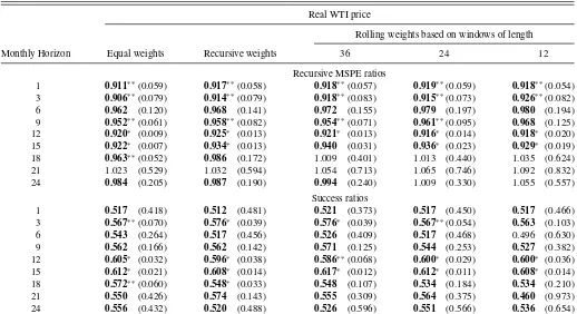
forecasting models. Each model receives weight 1/6 throughout. There is clear evidence of reductions in the MSPE relative to the no-change forecast up to a horizon of 18 months. The highest reduction is 9%. At horizons of 21 and 24 months, the equal-weighted forecast combination has an MSPE about as high as the no-change forecast. The equal-weighted forecast combination also has significant directional accuracy at horizons as long as 18 months. The highest success ratio is 65%. It is worth pointing out that some of the models included in the forecast combination achieve even larger gains at some horizons, but none produce consistently large accuracy gains across all horizons up to 18 months. This pattern of results is not specific to the real U.S. refiner’s acquisition cost for crude oil imports. The first column inTable 1(b)illustrates that similar, if somewhat weaker, results hold when forecasting the real WTI price. The reductions in the recursive MSPE are as high as 9% and the success ratios are as high as 61% and often statistically significant.
An obvious question is whether we can improve on these re-sults by weighting each model based on its recent forecasting
success. The second column inTable 1(a)shows that the
fore-cast combination based on recursively estimated inverse MSPE weights again systematically reduces the recursive MSPE at all horizons but horizon 21; in the latter case, it is almost as accurate as the no-change forecast. Overall the results are similar to those in the first column, but there is a slight reduction in accuracy. For example, the reductions in the recursive MSPE tend to be slightly lower. The largest reduction is 9%. The highest success ratio drops to 63%, and the degree of statistical significance is lower than when using equal weights. A similar slight reduc-tion of the forecasting accuracy can be observed in the second
column ofTable 1(b)for the real WTI price.
Recursively constructed forecast combination weights may not be optimal when dealing with smooth structural change in the global oil market. In the latter case, a more natural approach would be to use rolling windows in estimating the weights. An obvious question concerns the length of these windows. The more pronounced the structural change (or the less stable the individual forecasting models), the shorter the window length should be. At the same time, the window cannot be too short without the estimates of the weights becoming too noisy. In Table 1(a)we experiment with three window lengths: 36, 24,
and 12 months. The remaining columns in Table 1(a) show
that, while the results for the real refiners’ acquisition cost for imports remain remarkably robust across specifications, the use of rolling weights tends to undermine forecast accuracy. The shorter is the window length, the less accurate are the results.
The same pattern can be seen for the real WTI price inTable
1(b).
Overall, neither recursively constructed weights nor weights based on rolling windows of data can be recommended. The rea-son for this perhaps unexpected result is that these weights must
be constructed based on the fit of the model estimatedh+6
periods ago, wherehdenotes the forecast horizon in months,
and the additional delay of 6 months refers to the delays in the availability of reliable data. Although one could instead construct weights based on the nowcasts for data that are not re-leased yet and based on preliminary data to the extent available, we found that this strategy does not improve forecast accuracy and cannot be recommended. It can be shown that if forecasters
had access to the ex-post revised data in constructing forecast combination weights, the accuracy of the combination of real-time forecasts would increase considerably at all horizons. This point is moot, however, because this information is not available in real time, making equal-weighted forecast combinations the preferred choice in practice.
4. SENSITIVITY ANALYSIS
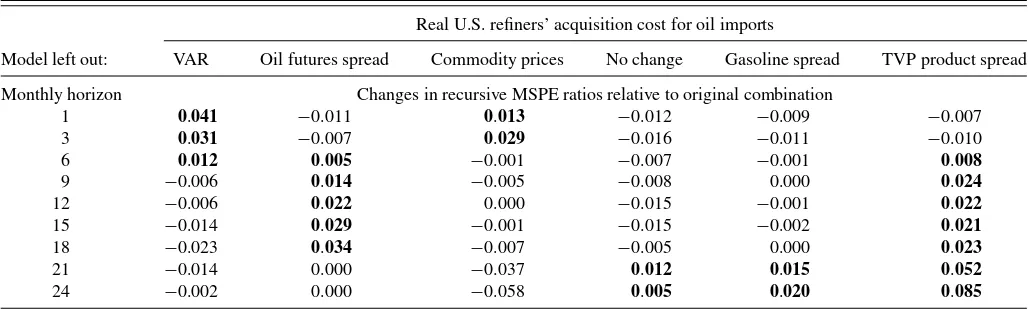
Our baseline combination involves six forecasting models. A question of practical interest is whether all of these models are required or whether the set of models may be reduced further. This question may be addressed by recomputing the accuracy of the forecast combination, having eliminated one model at a time from the equal-weighted forecast combination, as shown in Table 2. In each case, the weights are accordingly set to 1/5. Our
point of departure is the result in the first column ofTable 1(a).
Evidence that dropping one of the six models systematically lowers the recursive MSPE ratio would be an indication that this model ought to be eliminated from the forecast combination, if we care about the MSPE outcomes. We illustrate this approach inTable 2for the case of the real U.S. refiners’ acquisition cost for oil imports.
The first column ofTable 2shows that leaving out the VAR
model all else equal raises the MSPE ratio compared with the
first column inTable 1(a)at short horizons, reaffirming our
de-cision to include this model in the forecast combination, while lowering it at longer horizons. The second and third columns of Table 2provide evidence that the futures-based forecast helps improve the accuracy of the forecast combination at intermedi-ate horizons, while the forecast based on the non-oil commodity price model contributes at short horizons. In sharp contrast, the fourth column shows that the recursive MSPE may be lowered at all but the last two forecast horizons, if we eliminate the no-change model from the forecast combination. This result
con-tradicts the rationale we provided in Section2for including the
no-change forecast in the forecast combination. A similar sys-tematic improvement in the recursive MSPE can be observed after dropping the gasoline spread model in the fifth column, but not for the TVP product spread model in the last column, which contributes to the overall forecast accuracy especially at longer horizons. This evidence suggests that, at horizons up to 18 months, the gasoline spread model adds nothing beyond the predictive information in the TVP product spread model and should be eliminated from the forecast combination.
Similar results (not shown) also hold for the real WTI price, the main difference being that the VAR model contributes at horizons as long as 21 months, while the commodity price
model is useful only at short horizons. As in Table 2, the oil
futures spread model contributes to the accuracy of the fore-cast combination mainly at medium-term horizons, whereas the TVP product spread model contributes at medium and longer horizons.
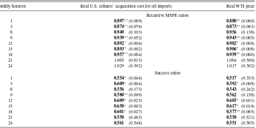
Table 3takes the analysis a step further by eliminating both the no-change forecast and the gasoline spread model from the equal-weighted forecast combination. The first column of Table 3confirms that eliminating both models further improves the accuracy of the forecast combination at most horizons up to 18 months, at the cost of worsening it at longer horizons.
Table 1a. Real-time forecast accuracy of baseline forecast combination based on all six forecasting models
Real U.S. refiners’ acquisition cost for oil imports
Rolling weights based on windows of length
Monthly horizon Equal weights Recursive weights 36 24 12
Recursive MSPE ratios
1 0.922∗∗(0.083) 0.927∗∗(0.090) 0.931∗∗(0.096) 0.929∗∗(0.085) 0.925∗∗(0.070)
3 0.906∗∗(0.072) 0.912∗∗(0.076) 0.916∗∗(0.079) 0.919∗∗(0.077) 0.919∗∗(0.057)
6 0.957∗∗(0.087) 0.964 (0.104) 0.966 (0.107) 0.976 (0.159) 0.971 (0.121)
9 0.948∗ (0.046) 0.955∗∗(0.066) 0.954∗∗(0.062) 0.961∗∗(0.086) 0.966 (0.108)
12 0.912∗ (0.004) 0.918∗ (0.007) 0.917∗ (0.009) 0.916∗ (0.009) 0.922∗ (0.010)
15 0.913∗ (0.003) 0.922∗ (0.005) 0.929∗ (0.014) 0.927∗ (0.011) 0.946∗ (0.026)
18 0.962∗∗(0.054) 0.979 (0.135) 1.002 (0.348) 1.002 (0.348) 1.023 (0.545)
21 1.025 (0.560) 1.030 (0.601) 1.051 (0.725) 1.058 (0.743) 1.110 (0.878)
24 0.992 (0.263) 0.987 (0.196) 0.991 (0.228) 1.000 (0.282) 1.043 (0.528)
Success ratios
1 0.570∗ (0.026) 0.558∗∗(0.054) 0.562∗ (0.039) 0.558∗∗(0.055) 0.566∗∗(0.050)
3 0.588∗ (0.028) 0.592∗ (0.020) 0.588∗ (0.023) 0.592∗ (0.018) 0.592∗ (0.021)
6 0.556 (0.192) 0.535 (0.336) 0.539 (0.307) 0.522 (0.437) 0.491 (0.664)
9 0.575 (0.121) 0.575 (0.105) 0.562 (0.170) 0.558 (0.176) 0.527 (0.370)
12 0.614∗ (0.019) 0.614∗ (0.010) 0.609∗ (0.017) 0.600∗ (0.019) 0.627∗ (0.005)
15 0.645∗ (0.004) 0.626∗ (0.004) 0.630∗ (0.006) 0.640∗ (0.000) 0.612∗ (0.005)
18 0.611∗ (0.016) 0.553∗ (0.044) 0.539 (0.142) 0.519 (0.242) 0.519 (0.289)
21 0.550 (0.419) 0.564 (0.232) 0.569 (0.319) 0.564 (0.452) 0.460 (0.965)
24 0.566 (0.412) 0.531 (0.523) 0.556 (0.544) 0.566 (0.495) 0.520 (0.761)
NOTES: The models are described in the text. Boldface indicates improvements relative to the no-change forecast. The statistical significance of the MSPE reductions cannot be assessed because none of the currently available tests of equal predictive accuracy applies in this setting. We nevertheless reportp-values in parentheses based on the test of Clark and West (2007). We also reportp-values for the Pesaran and Timmermann (2009) test for the null hypothesis of no directional accuracy.∗denotes significance at the 5% level and∗ ∗at the 10% level.
Table 1b. Real-time forecast accuracy of baseline forecast combination based on all six forecasting models
Real WTI price
Rolling weights based on windows of length
Monthly Horizon Equal weights Recursive weights 36 24 12
Recursive MSPE ratios
1 0.911∗∗(0.059) 0.917∗∗(0.058) 0.918∗∗(0.057) 0.919∗∗(0.059) 0.918∗∗(0.054)
3 0.906∗∗(0.079) 0.914∗∗(0.079) 0.918∗∗(0.083) 0.915∗∗(0.073) 0.926∗∗(0.082)
6 0.962 (0.120) 0.968 (0.141) 0.972 (0.155) 0.979 (0.197) 0.980 (0.194)
9 0.952∗∗(0.061) 0.958∗∗(0.082) 0.954∗∗(0.071) 0.961∗∗(0.095) 0.968 (0.125)
12 0.920∗ (0.009) 0.925∗ (0.013) 0.921∗ (0.013) 0.916∗ (0.014) 0.918∗ (0.020)
15 0.922∗ (0.007) 0.934∗ (0.013) 0.940 (0.031) 0.936∗ (0.023) 0.929∗ (0.019)
18 0.963∗∗(0.052) 0.986 (0.172) 1.009 (0.401) 1.013 (0.440) 1.035 (0.624)
21 1.023 (0.529) 1.032 (0.594) 1.054 (0.713) 1.065 (0.746) 1.092 (0.832)
24 0.984 (0.205) 0.987 (0.190) 0.994 (0.240) 1.009 (0.330) 1.055 (0.557)
Success ratios
1 0.517 (0.418) 0.512 (0.481) 0.521 (0.373) 0.517 (0.450) 0.517 (0.466)
3 0.567∗∗(0.070) 0.576∗ (0.039) 0.576∗ (0.039) 0.567∗∗(0.054) 0.563 (0.103)
6 0.543 (0.264) 0.517 (0.456) 0.526 (0.409) 0.517 (0.468) 0.496 (0.630)
9 0.562 (0.166) 0.562 (0.142) 0.571 (0.125) 0.544 (0.253) 0.527 (0.382)
12 0.605∗ (0.032) 0.596∗ (0.038) 0.586∗∗(0.068) 0.600∗ (0.029) 0.600∗ (0.036)
15 0.612∗ (0.021) 0.608∗ (0.014) 0.617∗ (0.012) 0.612∗ (0.011) 0.608∗ (0.014)
18 0.572∗∗(0.060) 0.548∗ (0.033) 0.548 (0.107) 0.534 (0.184) 0.534 (0.210)
21 0.550 (0.426) 0.574 (0.143) 0.555 (0.309) 0.564 (0.375) 0.460 (0.973)
24 0.556 (0.432) 0.520 (0.488) 0.526 (0.596) 0.551 (0.566) 0.536 (0.654)
NOTES: The models are described in the text. Boldface indicates improvements relative to the no-change forecast. The statistical significance of the MSPE reductions cannot be assessed because none of the currently available tests of equal predictive accuracy applies in this setting. We nevertheless reportp-values in parentheses based on the test of Clark and West (2007). We also reportp-values for the Pesaran and Timmermann (2009) test for the null hypothesis of no directional accuracy.∗denotes significance at the 5% level and∗ ∗at the 10% level.
Table 2. Changes in real-time recursive MSPE ratios of “leave-one-out” forecast combinations with equal weights
Real U.S. refiners’ acquisition cost for oil imports
Model left out: VAR Oil futures spread Commodity prices No change Gasoline spread TVP product spread
Monthly horizon Changes in recursive MSPE ratios relative to original combination
1 0.041 −0.011 0.013 −0.012 −0.009 −0.007
3 0.031 −0.007 0.029 −0.016 −0.011 −0.010
6 0.012 0.005 −0.001 −0.007 −0.001 0.008
9 −0.006 0.014 −0.005 −0.008 0.000 0.024
12 −0.006 0.022 0.000 −0.015 −0.001 0.022
15 −0.014 0.029 −0.001 −0.015 −0.002 0.021
18 −0.023 0.034 −0.007 −0.005 0.000 0.023
21 −0.014 0.000 −0.037 0.012 0.015 0.052
24 −0.002 0.000 −0.058 0.005 0.020 0.085
NOTES: The models are described in the text. Boldface indicates increases relative to the MSPE ratio in column (1) ofTable 1. Increases mean that the model left out would have improved forecast accuracy if included, whereas decreases mean that it would have worsened forecast accuracy. The statistical significance of the MSPE reductions cannot be assessed because none of the currently available tests of equal predictive accuracy applies in this setting.
A forecast combination consisting only of the VAR model, the commodity price model, the oil futures spread model, and the TVP product spread model, has lower recursive MSPE than the no-change forecast at all horizons from 1 month to 18 months. The reductions in the MSPE range from 4% to 13%. The im-provements in directional accuracy are statistically significant at all but one horizon and range from 55% to 65%, depending on the horizon. Similar results hold for the real WTI price, as shown
in the second column ofTable 3, albeit with somewhat lower
directional accuracy. The highest success ratio is still 62%, but the directional accuracy is statistically significant at only three of the first seven horizons considered.
The evidence inTable 1(a)and1(b)and inTable 3shows that
there is a practical alternative to the construction of judgmental forecasts of the real price of oil. Whether the combinations in Table 3are preferred relative to those inTable 1(a)and1(b), de-pends on how much we care about forecasting beyond a horizon of 18 months. Either way, an important question is whether the recursive MSPE reductions are driven by one or two unusual
episodes in the data or whether they are more systematic.
Fig-ure 1addresses this question by plotting the recursive MSPE ratio at each horizon for the evaluation period since 1997. We disregard the earlier MSPE ratios for being based on too short a recursive evaluation period to be considered reliable. For illus-trative purposes we focus on the real U.S. refiners’ acquisition cost for crude oil imports and equal weights as in the first
col-umn ofTable 1(a). Very similar results apply when using the
equal-weighted combination in the first column ofTable 3. The
plots show the evolution of the recursive MSPE ratios over time. The last observation of each plot corresponds to the entries in
the first column ofTable 1(a).
Figure 1 illustrates that at horizons of 1 and 3 the equal-weighted forecast combination has been consistently more ac-curate than the no-change forecast throughout the entire evalu-ation period since 1997. Similar results hold at horizons of 12, 15, and 18 months, but at horizons of 6 and 9 months there is evidence of the no-change forecast having been slightly more accurate early in the sample during 1997–2001. This pattern is consistent with the underlying regression estimates becoming more reliable as the estimation window lengthens. It may also
reflect the fact that the usefulness of economic fundamentals as predictors tends to be concentrated at shorter horizons, whereas that of product spreads tends to be most pronounced at horizons of 1 year and beyond, effectively limiting the sources of predic-tive information available at horizons of 6 and 9 months. Be that as it may, since 2001, the forecast combination has consistently been more accurate than the no-change forecast at all horizons between 1 month and 18 months.
The accuracy of the equal-weighted forecast combination at horizons of 21 months and 24 months is more erratic. On the one hand, relatively large recursive MSPE reductions occurred dur-ing 2003–2009, at the time of the Great Surge in oil prices driven by a booming world economy (see, e.g., Kilian and Murphy 2014). On the other hand, there are times when the no-change forecast has been more accurate. In the latter case, however, the recursive MSPE differences have rarely exceeded 5%. Thus, the
analysis inFigure 1lends further credence to the overall results
reported inTable 1(a)and1(b)and inTable 3.
5. EXTENSIONS TO QUARTERLY HORIZONS
As mentioned earlier, the EIA forecasts not only the monthly price of oil, but also quarterly averages. The construction of quarterly forecasts has been studied in depth in Baumeister and Kilian (2014a), who showed that the most accurate forecasts of the quarterly real price of oil are typically obtained by aggre-gating forecasts from models estimated at monthly frequency to quarterly frequency. For example, the average of the January, February, and March forecasts generated in December of the preceding year would constitute the forecast for the first quarter of the subsequent year.
There are two ways of proceeding. One method is first to construct forecast combinations of the forecasts generated each month for the monthly horizons 1 through 24 (similar to the
results shown in Tables 1(a),1(b), and3) and then to
aggre-gate the resulting monthly forecasts by quarter. This approach has the advantage that the monthly combination forecasts are fully consistent with the quarterly combination forecasts. An al-ternative method is to aggregate the monthly forecasts for each
1998 2000 2002 2004 2006 2008 2010 2012
1998 2000 2002 2004 2006 2008 2010 2012 0.7
1998 2000 2002 2004 2006 2008 2010 2012 0.7
1998 2000 2002 2004 2006 2008 2010 2012 0.7
1998 2000 2002 2004 2006 2008 2010 0.7
1998 2000 2002 2004 2006 2008 2010 0.7
1998 2000 2002 2004 2006 2008 2010 0.7
1998 2000 2002 2004 2006 2008 2010 0.7
1998 2000 2002 2004 2006 2008 2010 0.7
Figure 1. Real-time recursive MSPE ratio relative to no-change forecast for refiner’s acquisition cost for oil imports: Equal-weighted combination of all six forecasting models. NOTES: Results based on the forecast combination shown inTable 3. A ratio below 1 indicates an improvement relative to the no-change forecast. The plot shows the evolution of the recursive MSPE ratio over time for the forecast evaluation period since 1997. This increases the reliability of the MSPE estimates and allows the MSPE ratio to stabilize.
Table 3. Real-time forecast accuracy of forecast combination with equal weights after dropping the no-change forecast and gasoline spread forecast
Monthly horizon Real U.S. refiners’ acquisition cost for oil imports Real WTI price
Recursive MSPE ratios
1 0.897∗∗(0.089) 0.880∗∗(0.060)
3 0.874∗∗(0.078) 0.873∗∗(0.083)
6 0.949 (0.103) 0.956 (0.136)
9 0.939∗∗(0.052) 0.943∗∗(0.065)
12 0.892∗ (0.004) 0.902∗ (0.008)
15 0.893∗ (0.002) 0.906∗ (0.006)
18 0.957∗∗(0.064) 0.959∗∗(0.060)
21 1.065 (0.613) 1.064 (0.580)
24 1.029 (0.392) 1.017 (0.302)
Success ratios
1 0.554∗ (0.044) 0.517 (0.353)
3 0.609∗ (0.004) 0.592∗ (0.009)
6 0.556 (0.173) 0.543 (0.242)
9 0.580∗∗(0.099) 0.562 (0.156)
12 0.609∗ (0.023) 0.605∗ (0.031)
15 0.650∗ (0.003) 0.617∗ (0.018)
18 0.601∗ (0.027) 0.577∗∗(0.065)
21 0.550 (0.483) 0.550 (0.521)
24 0.561 (0.548) 0.551 (0.565)
NOTES: The models are described in the text. Boldface indicates improvements relative to the no-change forecast. The statistical significance of the MSPE reductions cannot be assessed because none of the currently available tests of equal predictive accuracy applies in this setting. We nevertheless reportp-values in parentheses based on the test of Clark and West (2007). We also reportp-values for the Pesaran and Timmermann (2009) test for the null hypothesis of no directional accuracy.∗denotes significance at the 5% level and∗ ∗at the 10% level.
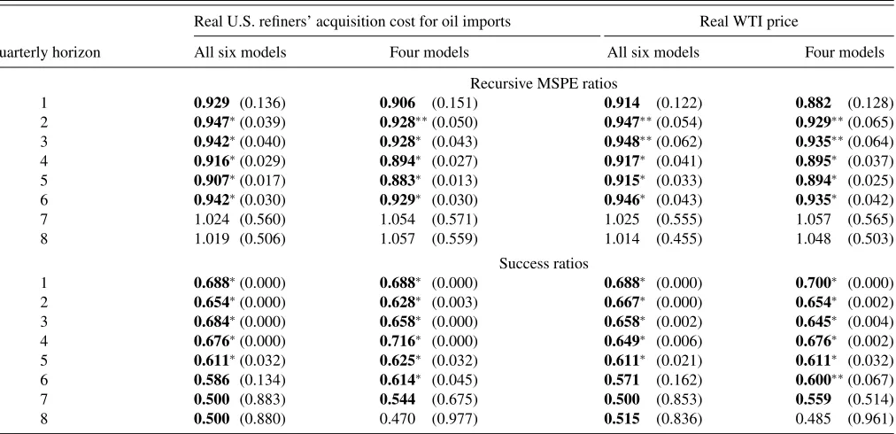
Table 4. Real-time forecast accuracy of equal-weighted forecast combinations at quarterly horizons
Real U.S. refiners’ acquisition cost for oil imports Real WTI price
Quarterly horizon All six models Four models All six models Four models
Recursive MSPE ratios
1 0.929 (0.136) 0.906 (0.151) 0.914 (0.122) 0.882 (0.128)
2 0.947∗(0.039) 0.928∗∗(0.050) 0.947∗∗(0.054) 0.929∗∗(0.065)
3 0.942∗(0.040) 0.928∗ (0.043) 0.948∗∗(0.062) 0.935∗∗(0.064)
4 0.916∗(0.029) 0.894∗ (0.027) 0.917∗ (0.041) 0.895∗ (0.037)
5 0.907∗(0.017) 0.883∗ (0.013) 0.915∗ (0.033) 0.894∗ (0.025)
6 0.942∗(0.030) 0.929∗ (0.030) 0.946∗ (0.043) 0.935∗ (0.042)
7 1.024 (0.560) 1.054 (0.571) 1.025 (0.555) 1.057 (0.565)
8 1.019 (0.506) 1.057 (0.559) 1.014 (0.455) 1.048 (0.503)
Success ratios
1 0.688∗(0.000) 0.688∗ (0.000) 0.688∗ (0.000) 0.700∗ (0.000)
2 0.654∗(0.000) 0.628∗ (0.003) 0.667∗ (0.000) 0.654∗ (0.002)
3 0.684∗(0.000) 0.658∗ (0.000) 0.658∗ (0.002) 0.645∗ (0.004)
4 0.676∗(0.000) 0.716∗ (0.000) 0.649∗ (0.006) 0.676∗ (0.002)
5 0.611∗(0.032) 0.625∗ (0.032) 0.611∗ (0.021) 0.611∗ (0.032)
6 0.586 (0.134) 0.614∗ (0.045) 0.571 (0.162) 0.600∗∗(0.067)
7 0.500 (0.883) 0.544 (0.675) 0.500 (0.853) 0.559 (0.514)
8 0.500 (0.880) 0.470 (0.977) 0.515 (0.836) 0.485 (0.961)
NOTES: The four models are obtained by dropping the no-change forecast and gasoline-spread forecast from the set of models to be combined. The models are described in the text. Boldface indicates improvements relative to the no-change forecast. The statistical significance of the MSPE reductions cannot be assessed because none of the currently available tests of equal predictive accuracy applies in this setting. We nevertheless reportp-values in parentheses based on the test of Clark and West (2007). We also reportp-values for the Pesaran and Timmermann (2009) test for the null hypothesis of no directional accuracy.∗denotes significance at the 5% level and∗ ∗at the 10% level.
individual forecasting method first and then to construct forecast combinations on the resulting quarterly forecasts. In the case of equal-weighted forecast combinations, this distinction becomes
moot.Table 4shows results for quarterly equal-weighted
fore-cast combinations constructed in this manner. The benchmark is again the no-change forecast based on the most recent monthly real price of oil in each quarter.
Given the construction of the quarterly real price of oil as the average of the monthly prices, it is not possible to infer from the
results inTables 1(a),1(b), and3how accurate the combination
forecasts for the quarterly data will be. The MSPE of the latter also depends on the unknown covariance between the monthly
forecasts.Table 4shows that, nevertheless, the quarterly
equal-weighted forecast combination performs quite well for the real U.S. refiners’ acquisition cost for oil imports. The first column ofTable 4shows systematic reductions in the recursive MSPE at all horizons up to six quarters ranging from 5% to 8%. The directional accuracy ranges at these horizons ranges from 59% to 69% and is mostly highly statistically significant. Similar results are also obtained for the real WTI price in the same table.
Eliminating the no-change forecast and the gasoline spread
forecasting model as inTable 3further improves the accuracy of
the quarterly forecasts at horizons up to six quarters. The MSPE
reductions in the second column of Table 4 may be as high
as 12% and the success ratios as high as 72% and statistically significant throughout. Similar results hold for the real WTI price.
It is worth emphasizing that forecast combinations are not necessarily more accurate across all horizons than the best indi-vidual forecasting models. For example, the TVP product spread model can be shown to be more accurate than any of the forecast
combinations at horizons of 7 and 8 quarters. The key advan-tage of the forecast combination is that it provides insurance against any one model breaking down unexpectedly. As with all insurance, there is a cost involved. In this case, the cost is a potential loss of accuracy compared with the single-most accu-rate model at any one horizon. There is also a benefit, however. In this example, the benefit is that the forecast combination is more accurate than the TVP spread model at horizons of one and two quarters. Moreover, while the TVP spread model has high directional accuracy, much of that directional accuracy is not statistically significant, whereas the directional accuracy of the forecast combination usually is.
As in the case of the monthly forecasts, it is useful to exam-ine the evolution of the recursive MSPE ratios. The results are
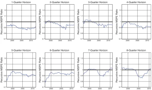
fully in line with the earlier evidence. Figure 2confirms that
at horizons of 1, 4, 5, and 6 quarters, the equal-weighted fore-cast combination has been consistently more accurate than the no-change forecast since 1997. At horizons of 2 and 3 quarters it has been consistently more accurate since 2000 and 2011, respectively. The performance at horizons of 7 and 8 quarters mirrors the results for the 21-month and 24-month horizons in Figure 1.
6. THE U.S. ENERGY INFORMATION ADMINISTRATION’S FORECASTS
So far we have not compared the accuracy of our preferred forecast combination directly with that of the EIA’s oil price forecasts. The reason is that these forecasts are not available for all horizons and data frequencies considered in our analysis. In this section, we evaluate the EIA oil price forecasts to the extent
2000 2005 2010
Figure 2. Real-time recursive MSPE ratio relative to no-change forecast for refiner’s acquisition cost for oil imports: Equal-weighted combination of all six forecasting models. Results based on the forecast combination shown inTable 4. A ratio below 1 indicates an improvement relative to the no-change forecast. The plot shows the evolution of the recursive MSPE ratio over time for the forecast evaluation period since 1997. This increases the reliability of the MSPE estimates and allows the MSPE ratio to stabilize.
that they are available for our evaluation period. The data source
for the EIA oil price forecasts is the EIA’sShort-Term Energy
Outlook. Most importantly for our purposes, this publication provides quarterly forecasts of the U.S. refiners’ acquisition cost for imports for horizons up to six quarters. Given the ir-regular pattern of the reports, however, consistent time series of quarterly forecasts dating back to 1991 can only be obtained
for horizons from one to four quarters ahead.6 This quarterly
time series allows us to gauge more directly the accuracy of the EIA’s forecasts and to compare their accuracy to that of alter-native forecasts. This question is interesting also because of the possibility that the EIA may have early access to oil market data allowing it to generate more accurate real-time forecasts than econometricians. We investigate this question below.
For the period 1991 to 1996, theShort-Term Energy Outlook
is issued every quarter. From 1997 onwards, the publication is released each month but only reports quarterly forecasts. The monthly publications are usually issued within the first two weeks of each month. The EIA updates its quarterly forecasts in each monthly report incorporating new information as it be-comes available. To make the forecast comparison meaningful it
6The corresponding monthly EIA forecasts of the U.S. refiners’ acquisition cost
are available only from 2004 onwards. They are reported for horizons up to 24 months. The EIA also reports monthly and quarterly WTI forecasts, but again the time series are short. Given the well-known sensitivity of forecast rankings to using small evaluation periods, we focus on the quarterly EIA forecasts of the U.S. refiners’ acquisition cost for imports that are available for the same long evaluation period already considered for our forecast combinations.
is important to match the information set of the EIA as closely as possible with our information set. Our default convention
(tim-ing convention (a) inTable 5) uses the end-of-quarter issues of
theShort-Term Energy Outlook(i.e., March, June, September, and December). The oil price reported for the current quarter is taken as the nowcast and the oil prices reported for the subse-quent quarters represent the forecasts. The corresponding real oil price forecasts are obtained by adjusting the nominal EIA oil price forecasts for expected inflation as already shown for the forecasts based on oil futures prices.
The first column of Table 5 shows that this EIA forecast
tends to be less accurate than the no-change forecast used as the default benchmark throughout the article. For example, at the one-quarter horizon, the EIA forecast has an MSPE that is 62% higher than the no-change forecast, while the preferred forecast
combination inTable 4has 9% lower MSPE than the benchmark.
At higher horizons, the extent of the losses from using the EIA forecast diminishes, but even at the four-quarter horizon, the EIA forecast is only about as accurate as the random walk, while the forecast combination is 11% more accurate. Nor does the EIA forecast have any statistically significant directional accuracy, in sharp contrast to our preferred forecast combination.
Under timing convention (a), the nowcast and forecasts effec-tively rely on information for the first two months of the current
quarter given that theShort-Term Energy Outlook is released
within the first two weeks of the third month of the quarter. While this timing accurately reflects the real-time availability of these forecasts, it implies that the EIA forecast has a slight
Table 5. Real-time forecast accuracy of EIA forecasts of the real U.S. refiners’ acquisition cost for imports
Timing convention (a) Timing convention (b) Timing convention (a)
Quarterly MSPE ratio relative to MSPE ratio relative to MSPE ratio relative to horizon no-change forecast no-change forecast EIA quarterly nowcast
1 1.618 (0.945) 0.996 (0.485) 0.926 (0.129)
2 1.291 (0.913) 1.122 (0.759) 1.113 (0.801)
3 1.086 (0.854) 1.046 (0.703) 1.049 (0.734)
4 1.004 (0.519) 0.956 (0.211) 0.948 (0.156)
Success ratio Success ratio Success ratio
1 0.374 (0.999) 0.602∗∗(0.058) 0.374 (0.999)
2 0.463 (0.767) 0.573 (0.174) 0.463 (0.767)
3 0.482 (0.730) 0.568 (0.207) 0.482 (0.730)
4 0.575 (0.151) 0.625∗ (0.027) 0.575 (0.151)
NOTES: The timing convention (a) for the EIA forecasts mimics a user of the EIA forecast who downloads the forecast at the end of each quarter at the same point in time when the model-based forecasts are constructed. The timing convention (b) allows the EIA an informational advantage of up to one month relative to the model-based forecasts. The comparison with the EIA quarterly nowcast is equivalent to the exercise for the nominal price of oil reported in Alquist et al. (2013). Boldface indicates improvements relative to the no-change forecast. The statistical significance of the success ratios is assessed based on the Pesaran and Timmermann (2009) test for the null hypothesis of no directional accuracy. The statistical significance of the MSPE reductions is assessed based on the Diebold and Mariano (1995) test. Thep-values are shown in parentheses.∗denotes significance at the 5% level and∗ ∗at the 10% level.
tional disadvantage compared with model-based forecasts. One way of gauging how much of a difference this fact makes is to evaluate the EIA forecast under a different timing convention
(timing convention (b) inTable 5). The proposal is to rely instead
on the issue of theShort-Term Energy Outlookthat appears in
the first month of the following quarter (i.e., April, July, Octo-ber, and January). Under this convention, the price reported for the previous quarter (e.g., the Q1 price in the April issue) is con-sidered the nowcast, and the price quoted for the current quarter (e.g., Q2 in the April issue) is the 1-quarter-ahead forecast.
Although this alternative convention gives the EIA fore-cast an informational advantage of up to one month rela-tive to model-based oil price forecasts, the second column of Table 5shows that even with that informational advantage the EIA forecast is never significantly more accurate than the no-change forecast with MSPE ratios as high as 1.12 at some hori-zons. There is some directional accuracy, but lower than for the preferred forecast combination and usually not statistically significant. This evidence suggests that the EIA’s forecasts are
systematically less accurate than our forecast combinations at all four horizons, even after controlling for informational delays associated with the timing of the releases of the EIA forecasts.
These results are clearly even less favorable to the EIA fore-cast than those reported in Alquist, Kilian, and Vigfusson (2013) for selected quarterly horizons. The reason is that in Alquist, Kil-ian, and Vigfusson (2013) the EIA forecasts were compared with the EIA’s own quarterly nowcast, as shown in the third column of Table 5under timing convention (a), rather than the no-change forecast from the real-time data base. As subsequently shown in Baumeister and Kilian (2014a) no-change forecasts based on quarterly nowcasts are distinctly less accurate than quarterly no-change forecasts based on the most recent monthly value of the price of oil, which explains the much higher MSPE ratio of
the EIA forecast in the first column ofTable 5. It is the latter
result that provides an accurate representation of the forecasting ability of the EIA forecast.
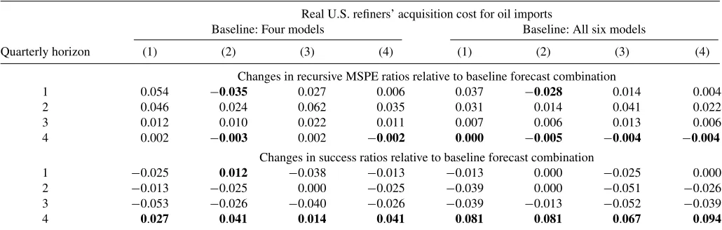
To summarize, the EIA forecast appears systematically less accurate compared with the preferred forecast combination
Table 6. Changes in real-time recursive MSPE ratios after including the EIA forecasts in the forecast combination
Real U.S. refiners’ acquisition cost for oil imports
Baseline: Four models Baseline: All six models
Quarterly horizon (1) (2) (3) (4) (1) (2) (3) (4)
Changes in recursive MSPE ratios relative to baseline forecast combination
1 0.054 −0.035 0.027 0.006 0.037 −0.028 0.014 0.004
2 0.046 0.024 0.062 0.035 0.031 0.014 0.041 0.022
3 0.012 0.010 0.022 0.011 0.007 0.006 0.013 0.006
4 0.002 −0.003 0.002 −0.002 0.000 −0.005 −0.004 −0.004
Changes in success ratios relative to baseline forecast combination
1 −0.025 0.012 −0.038 −0.013 −0.013 0.000 −0.025 0.000
2 −0.013 −0.025 0.000 −0.025 −0.039 0.000 −0.051 −0.026
3 −0.053 −0.026 −0.040 −0.026 −0.039 −0.013 −0.052 −0.039 4 0.027 0.041 0.014 0.041 0.081 0.081 0.067 0.094
NOTES: Boldface indicates improvement in forecast accuracy resulting from the inclusion of EIA forecasts in the baseline forecast combination. Specification (1) adds the EIA forecast based on timing convention (a) underlyingTable 5; (2) adds the EIA forecast based on timing convention (b) underlyingTable 5; (3) adds both EIA forecasts; (4) includes an equal-weighted average of the EIA forecasts based on timing conventions (a) and (b) in the forecast combination.