Full Terms & Conditions of access and use can be found at
http://www.tandfonline.com/action/journalInformation?journalCode=ubes20
Download by: [Universitas Maritim Raja Ali Haji] Date: 11 January 2016, At: 19:17
Journal of Business & Economic Statistics
ISSN: 0735-0015 (Print) 1537-2707 (Online) Journal homepage: http://www.tandfonline.com/loi/ubes20
Testing the Diagonality of a Large Covariance
Matrix in a Regression Setting
Wei Lan, Ronghua Luo, Chih-Ling Tsai, Hansheng Wang & Yunhong Yang
To cite this article: Wei Lan, Ronghua Luo, Chih-Ling Tsai, Hansheng Wang & Yunhong Yang
(2015) Testing the Diagonality of a Large Covariance Matrix in a Regression Setting, Journal of Business & Economic Statistics, 33:1, 76-86, DOI: 10.1080/07350015.2014.923317
To link to this article: http://dx.doi.org/10.1080/07350015.2014.923317
Accepted author version posted online: 12 Jun 2014.
Submit your article to this journal
Article views: 172
View related articles
Testing the Diagonality of a Large Covariance
Matrix in a Regression Setting
Wei L
ANStatistics School and Center of Statistical Research, Southwestern University of Finance and Economics, Chengdu 610072, P. R. China
Ronghua L
UOSchool of Finance, Southwestern University of Finance and Economics, Chengdu 610072, P. R. China ([email protected])
Chih-Ling T
SAIGraduate School of Management, University of California–Davis, Davis, CA 95616
Hansheng W
ANGand Yunhong Y
ANGGuanghua School of Management, Peking University, Peking, P. R. China
In multivariate analysis, the covariance matrix associated with a set of variables of interest (namely response variables) commonly contains valuable information about the dataset. When the dimension of response variables is considerably larger than the sample size, it is a nontrivial task to assess whether there are linear relationships between the variables. It is even more challenging to determine whether a set of explanatory variables can explain those relationships. To this end, we develop a bias-corrected test to examine the significance of the off-diagonal elements of the residual covariance matrix after adjusting for the contribution from explanatory variables. We show that the resulting test is asymptotically normal. Monte Carlo studies and a numerical example are presented to illustrate the performance of the proposed test.
KEY WORDS: Bias-corrected test; Diagonality test; High-dimensional data; Multivariate analysis.
1. INTRODUCTION
Covariance estimation is commonly used to study relation-ships among multivariate variables. Important applications in-clude, for example, graphical modeling (Edwards2000; Drton and Perlman2004), longitudinal data analysis (Diggle and Ver-byla1998; Smith and Kohn2002), and risk management (Ledoit and Wolf2004) among others. The total number of parameters needed for specifying a covariance matrix of a multivariate vec-tor with dimensionpisp(p+1)/2. When the sample sizenis less thanp, the large number of covariance parameters can sig-nificantly degrade the statistical efficiency of the usual sample covariance estimator, which makes interpretation difficult. It is, therefore, important to select the covariance structure so that the number of parameters needing to be estimated is reduced and an easy interpretation can be obtained.
There are a number of regularized estimation methods which have recently been developed to address this issue; current research has focused particularly on identifying various sparse structures; see, for example, Huang et al. (2006), Meinshausen and B¨uhlmann (2006), Lam and Fan (2009), Zhang and Leng (2012), and Leng and Tang (2012). While many novel meth-ods have been developed for covariance estimations, there has not yet been much discussion focusing on statistical tests of the covariance structure. In addition, the classical test statistics developed by John (1971), Nagao (1973), and Anderson (2003) are not applicable for high-dimensional data, since the spectral analysis of the sample covariance matrix is inconsistent under a high-dimensional setup (Bai and Silverstein2005). Efforts to
address this problem have led to various tests to determine if the covariance matrix is an identity or a diagonal matrix; see, for example, Srivastava (2005) and Chen, Zhang, and Zhong (2010). It is noteworthy that Chen, Zhang, and Zhong’s (2010) test allows forp→ ∞as n→ ∞without imposing the nor-mality assumption; thus it is quite useful for microarray studies (Efron2009; Chen, Zhang, and Zhong 2010). In addition, the aim of their test is to assess whether the covariance matrix ex-hibits sphericity (i.e., the matrix is proportional to the identity matrix; see Gleser1966, Anderson2003, and Onatski, Moreira, and Hallin2013) or identity without controlling for any covari-ates. As a result, Chen, Zhang, and Zhong’s (2010) test is not directly applicable for testing diagonality, in particular when explanatory variables are included in the model setting.
In practice, a set of variables of interest (namely, a set of re-sponse variables,Y ∈Rp) could be explained by another set of
explanatory variables,X∈Rd, in a linear form. For example,
Fama and French (1993,1996) introduced three variables to ex-plain the response of stock returns, and the resulting three-factor asset pricing model has been widely used in the fields of finance and economics. To assess the significance of the off-diagonal elements after adjusting for the contribution of explanatory
© 2015American Statistical Association Journal of Business & Economic Statistics January 2015, Vol. 33, No. 1 DOI:10.1080/07350015.2014.923317 Color versions of one or more of the figures in the article can be found online atwww.tandfonline.com/r/jbes. 76
variables, one can naturally adapt the aforementioned meth-ods to test whether the residual covariance matrix, cov{Y − E(Y|X)}, is diagonal or not. However, such an approach not only lacks theoretical justification but can also lead to inaccu-rate or misleading conclusions. This motivates us to develop a test for high-dimensional data in a regression setting to investi-gate whether the residual covariance matrix is diagonal or not. The resulting test can be applied in various fields, such as fi-nancial theory (Fan, Fan, and Lv2008) and microarray analysis (Chen, Zhang, and Zhong2010).
The rest of the article is organized as follows. Section2 intro-duces the model structure and proposes the bias-corrected test statistic. In addition, the theoretical properties of the resulting test are investigated. Section3 presents simulation studies to illustrate the finite sample performance of the proposed test. An empirical example is also provided to demonstrate the useful-ness of this test. Finally, we conclude the article with a brief discussion in Section4. All the technical details are left to the Appendix.
2. THEORETICAL ANALYSIS
2.1 Model Structure and A Test Statistic
LetYi =(Yi1, . . . , Yip)⊤ ∈Rpbe thep-dimensional response
vector collected for theith subject, where 1≤i≤n. For each subjecti, we further assume that there exists ad-dimensional ex-planatory vectorXi =(Xi1, . . . , Xid)⊤∈Rd. For the remainder of this article,dis assumed to be a fixed number, andp→ ∞as
n→ ∞with the possibility thatp≫n. Consider the following relationship betweenYiandXi,
Yi=B⊤Xi+Ei, (2.1)
where B=(β1, . . . , βp)∈Rd×p, βj =(βj1, . . . , βj d)⊤∈Rd
are unknown regression coefficients, andEi =(εi1, . . . , εip)⊤∈
Rp are independent and identically distributed vectors from a
multivariate normal distributions with mean vector zero and cov(Ei)==(σj1j2) for i=1, . . . , n. For the given dataset
Y=(Y1, . . . , Yn)⊤∈Rn×p and X=(X1, . . . , Xn)⊤∈Rn×d, we obtain the least squares estimator of the regression coef-ficient matrix B, B=(X⊤X)−1(X⊤Y)∈Rd×p. Subsequently,
the covariance matrixcan be estimated by ˆ =( ˆσj1j2), where
ˆ
σj1j2 =n
−1n
i=1εijˆ 1εijˆ 2, and ˆεij1and ˆεij2arej1th andj2th
com-ponents of ˆEi =Yi−Bˆ⊤Xi, respectively.
To test whether is a diagonal matrix or not, we consider the following null and alternative hypotheses,
H0:σj21j2=0 for anyj1=j2 vs.
H1:σj21j2>0 for somej1=j2. (2.2)
If the null hypothesis is correct, we should expect the abso-lute value of the off-diagonal element, ˆσj1j2, to be small for
any j1 =j2. Hence, we naturally consider the test statistic,
T∗=
j1<j2σˆ
2
j1j2. Under the null hypothesis, we can further
show that var1/2(T∗)=O(n−3/2p3/2) provided thatp/n
→ ∞, which motivates us to propose the following test statistic:
T =n3/2p−3/2 j1<j2
ˆ
σj21j2.
Clearly, one should reject the null hypothesis of diagonality if the value ofTis sufficiently large. However, we need to develop some theoretical justification to determine what value ofT is sufficiently large.
2.2 The Bias of Test Statistic
To understand the asymptotic behavior of the test statisticsT, we first compute the expectation ofTin the following theorem.
Theorem 1. Under the null hypothesisH0, we have
E(T)=1 2
n
−d n
1/2
n−d
p
1/2
pM12,p−M2,p
,
whereMκ,p =p−1pj=1σjjκ forκ =1 and 2.
The proof is given in Appendix A. Theorem 1 indicates that
E(T) is not exactly zero, which yields some bias. To further investigate the property of bias, we assume that Mκ,p→Mκ
as p→ ∞ for some |Mκ|<∞. Then, E(T)≈M2 1√np→
∞. As mentioned earlier, under the null hypothesis, we have var1/2(T∗)=O(n−3/2p3/2) ifp/n
→ ∞, which leads to var(T)=O(1). Accordingly, E(T)/var1/2(T)=O(√np)→ ∞, which suggests that T /{var(T)}1/2 is not asymptotically distributed as a standard normal random variable. This implies that we cannot ignore the bias due toT in asymptotic test, so we need to turn to methods of bias correction. To this end, we obtain an unbiased estimator ofE(T) as given below.
Theorem 2. UnderH0, we haveE(Bias)=E(T), where
Bias= n
3/2
2(n−d)p3/2
tr2( ˆ)−trˆ(2)
and ˆ(2)=σˆj2
1j2
. (2.3)
The proof is given in Appendix B. Theorem 2 shows that Bias is an unbiased estimator ofE(T). This motivates us to con-sider the bias-corrected statistic, T −Bias, whose asymptotic properties will be presented in the following section.
2.3 The Bias-Corrected (BC) Test Statistic
After adjustingTby its bias estimatorBias, we next study its variance.
Theorem 3. Assume that min{n, p} → ∞ and Mκ,p= p−1p
j=1σ κ
jj →Mκ for some constant|Mκ|<∞and for all κ ≤4. UnderH0, then var(T −Bias)=(n/p)M22,p+o(n/p).
The proof is given in Appendix C. Theorem 3 demonstrates that var(T −Bias)=O(n/p) and we can show that its asso-ciated term M2,p can be estimated by the following unbiased
estimators
M2,p=n2p−1[(n−d)2+2(n−d)]−1 p
j=1 ˆ
σjj2.
This drives us to consider the following bias-corrected (BC) test statistic:
Z= T −Bias
(n/p)1/2M 2,p
, (2.4)
whose asymptotic normality is established below.
Theorem 4. Assume that min{n, p} → ∞ and Mκ,p=
p−1p j=1σ
κ
jj →p Mκ for some constant |Mκ|<∞ and for
allκ ≤4. UnderH0, we haveZ→d N(0,1).
The proof is given in Appendix D. Theorem 4 indicates that the asymptotic null distribution ofZis standard normal, as long as min{n, p} → ∞. Applying this theorem, we are able to test the significance of the off-diagonal elements. Specifically, for a given significance levelα, we reject the null hypotheses of diag-onality ifZ > z1−α, whereZis the test statistics given in (2.4)
andzα stands for theαth quantile of a standard normal
distri-bution. Simulation studies, reported in the next section, suggest that such a testing procedure can indeed control the empirical size very well. It is noteworthy that Nagao’s (1973) diagonal test is valid only whenpis fixed. To accommodate high-dimensional data, Schott (2005) developed a testing procedure via the cor-relation coefficient matrix, which is useful if one is interested in testing whether cov(Y) is diagonal. However, it cannot be directly applied to test the diagonality of cov{Y −E(Y|X)}, unless the predictor dimension d is appropriately taken into consideration; see Remarks 2 and 3 for detailed discussions.
Remark 1.In multivariate models, researchers (e.g., Ander-son2003; Schott2005) have proposed various methods to test whether or not the covariance matrix is diagonal. It is interesting to recall that Anderson (2003) introduced the likelihood ratio test in the field of factor analysis as a method of examining the number of factors. In fact, identifying the number of common factors is similar to testing the diagonality of the covariance matrix of the specific factor. This leads us to propose our ap-proach for testing whether the covariance matrix of the error vector is diagonal, after controlling for the effect of explanatory variables.
Remark 2.By Theorem 2,Bias is an exactly unbiased esti-mator of T, and it contains the quantity (n−d). For the sake of simplicity, one may consider replacing (n−d) in the de-nominator of (2.3) bynso that the multiplier ofBias becomes
n1/2/(2p3/2). Under this replacement, however,E(T
−Bias)= 0 and it is of the orderO(n1/2/p1/2), which has the same order as (n/p)1/2M
2,pgiven in the denominator of (2.4). Hence, the
resulting test statistic is no longer distributed as a standard nor-mal. This suggests that the predictor dimension (i.e.,d) plays an important role for bias correction in our proposed BC-test statistic.
Remark 3.Although the BC-test in (2.4) shares some mer-its with the Schott (2005) test, there are three major differences given below. First, the BC-test considers min{p, n} → ∞, while the Schott test assumes thatp/n→cfor some finite constant
c >0. Second, the BC-test takes the predictors into considera-tion, which is not the focus of the Schott test. Third, the BC-test is obtained from the covariance matrix. In contrast, the Schott test is constructed via the correlation matrix and it is scale invari-ant. It is not surprising that the asymptotic theory of the Schott test is more sophisticated than that of the BC-test. According to
an anonymous referee’s suggestion as well as an important find-ing in Remark 2, we have carefully extended the Schott test to the model with predictorsZadj. We name it the adjusted Schott (AS) test, which is
Zadj=
(n−d)2(n−d+2) (n−d−1)p(p−1)
j1<j2
ˆ
rj21j2−p(p−1)
2(n−d)
,
(2.5)
where ˆrj1j2 =σjˆ1j2/{σˆ
1/2 j1j1σˆ
1/2
j2j2}. Following the techniques of
Schott (2005) with slightly complicated calculations, we are able to demonstrate thatZadjis asymptotic standard normal under the null hypothesis. However, its validity is established only when
p/n→cfor some finite constantc >0, as assumed by Schott (2005). In high-dimensional data withp≫n, the asymptotic theory is far more complicated and needs further investigation.
3. NUMERICAL STUDIES
3.1 Simulation Results
To evaluate the finite sample performance of the bias-corrected test, we conduct Monte Carlo simulations. We con-sider model (2.1), where the predictor Xi=(Xij) is gener-ated from a multivariate normal distribution withE(Xij)=0, var(Xij)=1, and cov(Xij1, Xij2)=0.5 for anyj1=j2. In
addi-tion, the regression coefficientsβj kare independently generated from a standard normal distribution. Moreover, the error vector
Ei=(εij) is generated as follows: (i) theεij are generated from
normal distributions with mean 0; (ii) the variance ofεij (i.e., σjj) is simulated independently from a uniform distribution on
[0,1]; (iii) the correlation betweenεij1 andεij2 for anyj1=j2 is fixed to be a constantρ.
We simulated 1000 realizations with a nominal level of 5%, each consisting of two sample sizes (n=100 and 200), three dimensions of multivariate responses (p=100, 500, and 1000), and four dimensions of explanatory variables (d =0, 1, 3, and 5). The value ofρ=0 corresponds to the null hypothesis. Schott (2005) developed a diagonal test in high-dimensional data un-derd=0. For the sake of comparison, we include the Schott (2005, sec.2) test by calculating the sample correlation with the estimated residualEi rather than the responseYi. In addition,
we consider the adjusted Schott test given in (2.5).
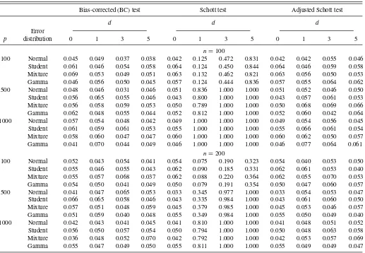
Under normal errors, Table 1 reports the sizes of the BC, Schott, and adjusted Schott tests. Whend=0, all three tests per-form well. However, the perper-formance of the Schott test deterio-rates withd >0. This indicates that the Schott test cannot be di-rectly applied to assess the diagonality of the residual covariance matrix after incorporating the contribution from explanatory variables. In contrast, after adjusting for the effective sample size fromnton−d, the performance of the adjusted Schott test be-comes satisfactory, which indicates that the predictor dimension dis indeed critical.Table 1also indicates that the BC test con-trols the empirical sizes well across the various sample sizes, di-mensions of response variables, and didi-mensions of explanatory variables. To examine their robustness, we also generated errors from the Student (t5), mixture (0.9N(0,1)+0.1N(0,32)), and Gamma(4,0.5) distributions. Table 1 shows that, under these error distributions, both tests control the empirical size
Table 1. The sizes of bias-corrected (BC), Schott and adjusted Schott tests for testingH0:ρ=0 with a nominal level of 5%
Bias-corrected (BC) test Schott test Adjusted Schott test
d d d
Error
p distribution 0 1 3 5 0 1 3 5 0 1 3 5
n=100
100 Normal 0.045 0.049 0.037 0.038 0.042 0.125 0.472 0.831 0.042 0.042 0.055 0.046 Student 0.061 0.046 0.054 0.058 0.064 0.124 0.450 0.844 0.064 0.046 0.059 0.058 Mixture 0.069 0.053 0.049 0.051 0.063 0.132 0.462 0.821 0.063 0.056 0.050 0.053 Gamma 0.046 0.056 0.050 0.045 0.057 0.124 0.444 0.836 0.057 0.055 0.064 0.062 500 Normal 0.048 0.046 0.031 0.046 0.051 0.836 1.000 1.000 0.051 0.052 0.046 0.050 Student 0.056 0.065 0.055 0.046 0.043 0.800 1.000 1.000 0.043 0.057 0.061 0.053 Mixture 0.056 0.058 0.059 0.053 0.050 0.789 1.000 1.000 0.050 0.068 0.069 0.066 Gamma 0.062 0.048 0.055 0.044 0.052 0.812 1.000 1.000 0.052 0.060 0.042 0.064 1000 Normal 0.057 0.054 0.048 0.042 0.049 1.000 1.000 1.000 0.049 0.054 0.056 0.045 Student 0.061 0.059 0.061 0.053 0.055 1.000 1.000 1.000 0.055 0.066 0.061 0.054 Mixture 0.058 0.060 0.047 0.047 0.060 1.000 1.000 1.000 0.060 0.062 0.050 0.057 Gamma 0.041 0.070 0.044 0.049 0.046 1.000 1.000 1.000 0.046 0.077 0.064 0.061
n=200
100 Normal 0.052 0.043 0.054 0.041 0.054 0.075 0.190 0.323 0.054 0.040 0.053 0.050 Student 0.055 0.046 0.055 0.043 0.062 0.090 0.185 0.331 0.062 0.061 0.053 0.040 Mixture 0.055 0.057 0.068 0.037 0.062 0.088 0.220 0.364 0.062 0.055 0.070 0.053 Gamma 0.054 0.050 0.041 0.049 0.050 0.079 0.191 0.354 0.050 0.047 0.060 0.057 500 Normal 0.041 0.047 0.065 0.053 0.033 0.345 0.977 1.000 0.033 0.054 0.053 0.047 Student 0.066 0.065 0.058 0.046 0.043 0.335 0.984 1.000 0.043 0.061 0.060 0.050 Mixture 0.057 0.051 0.048 0.059 0.045 0.379 0.985 1.000 0.045 0.053 0.046 0.057 Gamma 0.051 0.059 0.040 0.048 0.055 0.349 0.984 1.000 0.055 0.050 0.049 0.040 1000 Normal 0.042 0.043 0.041 0.045 0.041 0.810 1.000 1.000 0.041 0.048 0.051 0.052 Student 0.056 0.050 0.057 0.054 0.050 0.794 1.000 1.000 0.050 0.048 0.063 0.058 Mixture 0.036 0.048 0.052 0.070 0.042 0.792 1.000 1.000 0.042 0.053 0.057 0.069 Gamma 0.055 0.047 0.049 0.050 0.055 0.811 1.000 1.000 0.055 0.049 0.049 0.047
adequately. Finally, we investigate the power of the BC test and the AS test. For the sake of illustration, we consider only the case with normal errors,n=100, andd =1. Figure 1depicts the power functions for three dimensions of response variables (p=
100, 500,and 1000), respectively. It shows that the powers of the two tests are almost identical, and the power increases asp be-comes large. Since all simulation results forn=200 show a sim-ilar pattern, we do not report them here. In sum, both BC and AS tests are reliable and powerful, while the theoretical justification for the AS test needs further study as mentioned in Remark 3.
Finally, upon the suggestions of an AE and an anonymous referee, we have compared our proposed test with Chen, Zhang, and Zhong’s (2010) test and with Ledoit and Wolf’s (2002) test, which was mentioned in Onatski, Moreira, and Hallin (2013), for testing high-dimensional covariances via simulation studies withd =0. The results show that all these tests perform well in testing for identity, while the BC test is superior to Chen, Zhang, and Zhong’s and Ledoit and Wolf’s tests for testing diagonality. This finding is not surprising since those two tests are not developed for examining diagonality.
3.2 A Real Example
To further demonstrate the practical usefulness of our pro-posed method, we consider an important finance application. Specifically, we employ our method to address an critical
question: how many common factors (i.e., explanatory vari-ables) are needed to fully describe the covariance structure of security returns? By Trzcinka (1986), Brown (1989), and Con-nor and Korajczky (1993), this is one of the fundamental prob-lems in portfolio theory and asset pricing. To this end, we collect the data from a commercial database, which contains weekly re-turns for all of the stocks traded on the Chinese stock market during the period of 2008–2009. After eliminating those stocks with missing values, we obtain a total ofp=1058 stocks with sample sizen=103.
We consider as our explanatory variables, several of the fac-tors most commonly used in the finance literature to explain the covariance structure of stock returns. The first such factor is Xi1=market index, in this case, returns for the Shanghai Composite Index. The market index is clearly the most im-portant factor for stock returns because it reflects the overall performance of the stock market. As a result, it serves as the foundation for the Capital Asset Pricing Model (Sharpe1964; Lintner1965; Mossin1966). Empirical studies, however, have suggested that the market index alone cannot fully explain the correlation structure of stock returns. Fama and French (1993, 1996) proposed the three-factor model to address this prob-lem; they include the market index as well as two other factors which are denoted by Xi2= SMB andXi3=HML. Specifi-cally,Xi2measures the size premium (i.e., the difference in re-turns between portfolios of small capitalization firms and large
0.0
0.2
0.4
0.6
0.8
1.0
ρ
P
o
wer (%)
0 0.009 0.021 0.033 0.045 BC test AS test
p=100
0.0
0.2
0.4
0.6
0.8
1.0
ρ
P
o
wer (%)
0 0.009 0.021 0.033 0.045 BC test AS test
p=500
0.0
0.2
0.4
0.6
0.8
1.0
ρ
P
o
wer (%)
0 0.009 0.021 0.033 0.045 BC test AS test
p=1,000
Figure 1. Power functions for testingH0:ρ=0 with normal errors andn=100.
capitalization firms) and Xi3 is the book-to-market premium (i.e., the difference in returns between portfolios of high book-to-market firms and low book-book-to-market firms). Finally, re-cent advances in behavioral finance suggest that stock returns have nontrivial momentum, which is captured by the differ-ence in returns between portfolios of high and low prior re-turns. To this end, Jegadeesh and Titman (1993) and Carhart (1997) proposed the momentum factor, which is denoted by
Xi4.
In our analysis, we consider four nested models, M0=
∅,M1= {Xi1},M2= {Xi1, Xi2, Xi3}, and M3= {Xi1, Xi2,
Xi3, Xi4} and apply the proposed method to each candidate model; this gives test statistics of 20,560, 3357, 228, and 215, respectively. Similar results are obtained via the AS test. We draw two conclusions from these results. The first comes from observing the differences between these values. As expected, the Fama–French model (M2) improves enormously on both
the model with no predictors and the model with only the market index, and while the fourth factor (momentum) does improve on the Fama–French model, its contribution is clearly small. The proposed statistical method, therefore, provides additional confirmation that the Fama–French model is an extremely im-portant finance model, even in datasets withp > n. Second, the addition of a fourth factor still does not allows us to accept the null hypothesis of a diagonal covariance matrix. This suggests that there may be factors unique to the Chinese stock market which contribute significantly to the covariance structure. To explore this idea further, we applied the principle component method of factor analysis to the residuals ofM3and found that
the test statistic continued to decline with the inclusion of as many as 75 of the additional factors we identified. While this additional finding is interesting, it lacks of insightful financial
interpretations, and so we believe that further research on risk factors in the Chinese stock market is warranted.
4. DISCUSSIONS
In this article, we propose a bias-corrected test to assess the significance of the off-diagonal elements of a residual covari-ance matrix for high-dimensional data. This test takes into ac-count the information from explanatory variables, which broad-ens the application of covariance analysis. Although the results are developed in the context of a linear regression, it could cer-tainly be extended to nonparametric regressions; see, for exam-ple, Fan and Gijbels (1996), H¨ardle, Liang, and Gao (2000), and Xia (2008). In the theoretical development of our test statistic, we focus principally on the normal error assumption. It could, however, be useful to obtain a test for diagonality with weaker assumptions such as sub-Gaussian errors, although simulation studies show that the proposed test performs well for nonnormal errors. Moreover, it would be interesting to extend our test to the correlation matrix withd >0 and min{n, p} → ∞. Finally, a generalization of the test statistic to the case withd > ncould be of interest. In this context, the shrinkage regression estimates, for example, LASSO of Tibshirani (1996), SCAD of Fan and Li (2001), and Group LASSO of Yuan and Lin (2006), could be useful in developing a test statistic. Based on our limited studies, obtaining a shrinkage estimator ofBthat is consistent for variable selection will be important in extending our pro-posed test. With a consistently selected model, we believe that the usual OLS-type estimator and the theoretical development of the resulting test statistic can be achieved. Consequently, it is essential to develop an effective shrinkage method for both
d > nandn→ ∞.
APPENDIX A: PROOF OF THEOREM 1
To facilitate the proof, we will refer to the following lemmas, so we present them first. The proof of Lemma 2 follows directly from the proof of Lemma 3 in Magnus (1986). Its proof is therefore omitted.
Lemma A.1. Let U1 and U2 be twom×1 independent random
vectors with mean vector 0 and covariance matrixIm, where Im is
an m×m identity matrix. Then for any m×mprojection matrix
A, we have (a) E(U⊤
1AU1)=tr(A) and (b) E[(U1⊤AU2)2]=tr(A).
Further assumeU1 and U2 follow multivariate normal distributions,
then we have (c)E[(U⊤
Proof. The proofs of (a) and (b) are straightforward, and are there-fore omitted. In addition, results (d) and (e) can be directly obtained from Proposition 1 of Chen, Zhang, and Zhong (2010). As a result, we only need to show part (c). Using the fact that U⊤
1 AU2∈R1,
U⊤
1 AU1∈R1,U2⊤AU2∈R1,U1⊤AU2=U2⊤AU1, andU1 andU2are
mutually independent, we have
EU1⊤AU2
Using the fact thatU1 is a m-dimensional standard normal random
vector, we obtain U1 and U2 are independent identically distributed random
vari-ables and A is a projection matrix, the right-hand side of (A.1) is equal to tr(2A2
Lemma A.2. LetUbe anm×1 normally distributed random vector with mean vector 0 and covariance matrixIm, and letAbe am×m
symmetric matrix. Then, for the fixed integers, we have that,
E(U⊤AU)s
Proof of Theorem 1
Let εj=(ε1j, ε2j, . . . , εnj)⊤∈Rn for j=1, . . . , d. From the
regression model (2.1), we know that εj has mean 0 and
covari-ance matrix σjjI, whereI∈Rn×n is a n×n matrix. Furthermore,
This completes the proof.
APPENDIX B: PROOF OF THEOREM 2
By Lemma 1(a), we have thatE( ˆσjj)=n−1(n−d)σjj. Then, using
This, together with (A.2), implies that
n3/2
which completes the proof.
APPENDIX C: PROOF OF THEOREM 3
Note that var{T −Bias} =E{Bias2} +E{T2
} −2E{TBias}, where the right-hand side of this equation contains three components. They can be evaluated separately according to the following three steps.
}defined in Theorem 2, we then ob-tain
Case II: i1=i2, j1=j2, but i1=j1. Then, ˆσi1i1σˆj1j1σˆi2i2σˆj2j2=
Applying the same procedure as that used in Step 1, we computeE(T2)
according to the following three different cases.
Case I.i1,i2,j1, andj2are mutually different. Then, ˆσi1j1and ˆσj2j2
are mutually independent. By Lemma 1(b), we have
Eεi⊤1(I−H)εj1
Lemma 1(e), we obtain that
Eε⊤
Step 3. Finally we computeE{TBias}. After algebraic simplifica-tion, we obtain the following expression:
TBias=4−1n3(n−d)−1p−3
Similar to Steps 1 and 2, we consider three cases given below to calculate this quantity separately.
Case I.i1,i2,j1, andj2are mutually different. Then, ˆσi21j1, ˆσi2i2, and
ˆ
σj2j2are mutually independent. By Lemma 1(a) and 1(b), we have
Eε⊤
Accordingly, we obtain that Hence, the second and third terms in (C.15) are negligible as compared with the first term,nM2
2,p/p=O(n/p). Analogously, the last term
in (C.15) is also negligible sincep→ ∞. In sum, we have var(T − Bias)=nM2
2,p/p+o(n/p). This completes the proof.
APPENDIX D. PROOF OF THEOREM 4
To prove this theorem, we need to demonstrate (I.) (T −Bias)/var1/2(T
−Bias) is asymptotically normal; and (II.)
M2,p →pM2,p. Because (II) can be obtained by applying the same
tech-niques as in the proof of Lemma 2.1 of Srivastava (2005), we only fo-cus on (I). To show the asymptotic normality of (T −Bias)/var1/2(T
−
Bias), we need to employ the martingale central limit theorem; see Hall and Heyde (1980). To this end, we defineFr=σ{ε1, ε2, . . . , εr}, which
p,r|Fr−1). Accordingly, by the martingale central limit theorem
(Hall and Heyde1980), it suffices to show that
p
This can be done in three steps given below. In the first step, we obtain an analytical expression ofσ2
p,r, which facilitates subsequent technical
proofs. The second step demonstrates the first part of (D.2), while the last step verifies the second part of (D.2).
Step 1. Using the fact thatn1/2p3/2
To obtain the explicit expression ofσ2
p.r, we next calculate the three
terms on the right-hand side of (D.3) separately. The first term in (D.3). It is noteworthy that
Eε⊤i(I−H)εr
in the first term’s calculation. For the sake of simplic-ity, let {ε⊤
Because εr is a n-dimensional normal vector with mean 0
and variance σrrI, this leads to E(cgh|Fr−1)=σrr2
becauseI−H is a projection matrix. This, together with (D.4), leads
This completes the calculation of the major component of the first term in (D.3).
The second term in (D.3). Employing Lemma 1(d), we obtain that
(n−d)−2 by computing its major component,
Eε⊤
rrI. The above results lead to
Eε⊤i(I−H)εr
which completes the calculation of the major component of the third term. This, together with (D.3), (D.5), and (D.6), yields,
a martingale sequence, one can verify that E(σ2
p,1+σp,22+ · · · +
σ2
p,p)=var
T −Bias. Accordingly, we only need to show that var(pr=1σ2
p,r)/var2(T −Bias)→0. To this end, we focus on
calculat-ing var(pr=1σ2
p,r). Because Theorem 3 implies that var(T −Bias)=
O(np−1), (D.9) suggests that we can prove the first part of (D.2) by
demonstrating the following results:
(i) var
To prove Equation (i), we first note that
p
algebraic simplification, we have
var
where the last inequality is using the fact that {1− (n−d)−1
the right-hand side of (D.11) can be further bounded from infinity by
2n
This verifies the Equation (i) in (D.10).
We next show Equation (ii). Becauseap,r =rs=1p,s, we obtain
By Cauchy’s inequality, the right-hand side of the above inequality can be further bounded from infinity by
p2M2
Moreover, using the result that will be demonstrated in (D.13), we haveps=1E(4
p,s)=O(n
2p−3). This, together with the assumption,
M2,p →pM2with|M2|<∞, implies that the right-hand side of (D.12)
is the order ofO(np)=o(n3p), which completes the proof of Equation
(ii) in (D.10).
Step 3. We finally show the second part of (D.2). It is noteworthy that
whereAr=(I−H)εrεr⊤(I−H)−(n−d)−
1(I
−H){ε⊤
r (I−H)εr}
that is a symmetric matrix, and it is related to the current observationεr
only. Wheni=r, one can show that tr(Ar)=0 andE(ε⊤iArεi|εr)=0.
Using these results, we have
n2p6E4
In addition, one can verity by Lemma 2 that there exists constantsC1,
C2, andC3such that
After algebraic simplification, we obtain that
trA2r
where C4 is a positive constant and the last inequality is because
ε⊤
which proves the second part of (D.2) and thus completes the proof of Theorem 4.
ACKNOWLEDGMENTS
Wei Lan’s research was supported by the Fundamental Re-search Funds for the Central Universities, 14TD0046, and by National Natural Science Foundation of China (NSFC, 11401482). Hansheng Wang’s research was supported in part by National Natural Science Foundation of China (NSFC, 11131002, 11271032), Fox Ying Tong Education Foundation, the Business Intelligence Research Center at Peking University, and the Center for Statistical Science at Peking University. Yun-hong Yang’s research was supported by National Natural Sci-ence Foundation of China (NSFC, 71172027). Ronghua Luo’s research was supported by the National Natural Science Foun-dation of China (NSFC, 11001225). The authors are grateful to the Editor, the AE, and the anonymous referees for their insightful comments and constructive suggestions.
[Received October 2013. Revised March 2014.]
REFERENCES
Anderson, T. W. (2003),An Introduction to Multivariate Statistical Analysis
(3rd ed.), New York: Wiley. [76,78]
Bai, Z. D., and Silverstein, J. W. (2005),Spectral Analysis of Large Dimensional Random Matrices, Beijing: Scientific Press. [76]
Brown, S. J. (1989), “The Number of Factors in Security Returns,”The Journal of Finance, 44, 1247–1262. [79]
Carhart, M. M. (1997), “On Persistency in Mutual Fund Performance,”Journal of Finance, 52, 57–82. [80]
Chen, S. X., Zhang, L. X., and Zhong, P. S. (2010), “Tests for High Dimensional Covariance Matrices,”Journal of the American Statistical Association, 105, 810–819. [76,81]
Connor, G., and Korajczky, R. (1993), “A Test for the Number of Factors in an Approximate Factor Model,” The Journal of Finance, 48, 1263– 1291. [79]
Diggle, P., and Verbyla, A. (1998), “Nonparametric Estimation of Covariance Structure in Longitudinal Data,”Biometrics, 54, 401–415. [76]
Drton, M., and Perlman, M. (2004), “Model Selection for Gaussian Concentra-tion Graphs,”Biometrika, 91, 591–602. [76]
Edwards, D. M. (2000), Introduction to Graphical Modeling, New York: Springer. [76]
Efron, B. (2009), “Are a Set of Microarrays Independent of Each Other?”The Annals of Applied Statistics, 3, 992–942. [76]
Fama, E., and French, K. (1993), “Common Risk Factors in the Returns on Stocks and Bonds,”Journal of Financial Economics, 33, 3–56. [76,79] ——— (1996), “Multifactor Explanations of Asset Pricing Anomalies,”The
Journal of Finance, 51, 55–84. [76,79]
Fan, J., Fan, Y., and Lv, J. (2008), “High Dimensional Covariance Matrix Estimation Using a Factor Model,”Journal of Econometrics, 147, 186–197. [77]
Fan, J., and Gijbels, I. (1996),Local Polynomial Modeling and Its Applications, New York: Chapman and Hall. [80]
Fan, J., and Li, R. (2001), “Variable Selection via Nonconcave Penalized Like-lihood and Its Oracle Properties,”Journal of the American Statistical Asso-ciation, 96, 1348–1360. [80]
Gleser, L. J. (1966), “A Note on the Sphericity Test,”The Annals of Mathemat-ical Statistics, 37, 464–467. [76]
Hall, P., and Heyde, C. C. (1980),Martingale Limit Theory and Its Application, New York: Academic Press. [83]
H¨ardle, W., Liang, H., and Gao, J. (2000),Partially Linear Models, Heidelberg: Springer. [80]
Huang, J. Z., Liu, N., Pourahmadi, M., and Liu, L. (2006), “Covariance Selection and Estimation via Penalized Normal Likelihood,”Biometrika, 93, 85–98. [76]
Jegadeesh, N., and Titman, S. (1993), “Returns to Buying Winners and Selling Lowers: Implications for Stock Market Efficiency,”Journal of Finance, 48, 65–91. [80]
John, S. (1971), “Some Optimal Multivariate Test,”Biometrika, 59, 123–127. [76]
Lam, C., and Fan, J. (2009), “Sparsistency and Rates of Convergence in Large Covariance Matrices Estimation,”The Annals of Statistics, 37, 4254–4278. [76]
Ledoit, O., and Wolf, M. (2002), “Some Hypothesis Tests for the Covariance Matrix When the Dimension is Large Compared to the Sample Size,”The Annals of Statistics, 30, 1081–1102. [76]
——— (2004), “Honey, I Shrunk the Sample Covariance Matrix,”Journal of Portfolio Management, 4, 110–119. [76]
Leng, C., and Tang, C. (2012), “Sparse Matrix Graphical Models,”Journal of the American Statistical Association, 4, 1187–1200. [76]
Lintner, J. (1965), “The Valuation of Risky Assets and the Selection of Risky Investments in Stock Portfolios and Capital Budgets,”Review of Economics and Statistics, 47, 13–37. [79]
Magnus, J. R. (1986), “The Exact Moments of a Ratio of Quadratic Forms in Normal Variables,”Annals of Economics and Statistics, 4, 95–109. [81] Meinshausen, N., and B¨uhlmann, P. (2006), “High-Dimensional Graphs and
Variable Selection With the Lasso,”The Annals of Statistics, 34, 1436– 1462. [76]
Mossin, J. (1966), “Equilibrium in a Capital Asset Market,”Econometrika, 34, 768–783. [79]
Nagao, H. (1973), “On Some Test Criteria for Covariance Matrix,”The Annals of Statistics, 1, 700–709. [76]
Onatski, A., Moreira, M. J., and Hallin, M. (2013), “Asymptotic Power of Sphericity Tests for High Dimensional Data,”The Annals of Statistics, 41, 1055–1692. [76,79]
Schott, J. R. (2005), “Testing for Complete Independence in High Dimensions,”
Biometrika, 92, 951–956. [78]
Sharpe, W. (1964), “Capital Asset Prices: A Theory of Market Equilibrium Under Conditions of Risks,”Journal of Finance, 19, 425–442. [79] Smith, M., and Kohn, R. (2002), “Parsimonious Covariance Matrix Estimation
for Longitudinal Data,”Journal of the American Statistical Association, 97, 1141–1153. [76]
Srivastava, M. S. (2005), “Some Tests Concerning the Covariance Matrix in High Dimensional Data,”Journal of Japan Statistical Society, 35, 251–272. [76,83]
Tibshirani, R. J. (1996), “Regression Shrinkage and Selection via the LASSO,”
Journal of the Royal Statistical Society,Series B, 58, 267–288. [80]
Trzcinka, C. (1986), “On the Number of Factors in the Arbitrage Pricing Model,”
The Journal of Finance, 41, 347–368. [79]
Xia, Y. (2008), “A Multiple-Index Model and Dimension Reduction,”Journal of the American Statistical Association, 103, 1631–1640. [80]
Yuan, M., and Lin, Y. (2006), “Model Selection and Estimation in Regression With Grouped Variables,”Journal of the Royal Statistical Society,Series B, 68, 49–67. [80]
Zhang, W., and Leng, C. (2012), “A Moving Average Cholesky Factor Model in Covariance Modeling for Longitudinal Data,”Biometrika, 99, 141–150. [76]