Full Terms & Conditions of access and use can be found at
http://www.tandfonline.com/action/journalInformation?journalCode=ubes20
Download by: [Universitas Maritim Raja Ali Haji] Date: 13 January 2016, At: 00:26
Journal of Business & Economic Statistics
ISSN: 0735-0015 (Print) 1537-2707 (Online) Journal homepage: http://www.tandfonline.com/loi/ubes20
Hierarchical Models for Employment Decisions
Joseph B Kadane & George G Woodworth
To cite this article: Joseph B Kadane & George G Woodworth (2004) Hierarchical Models for Employment Decisions, Journal of Business & Economic Statistics, 22:2, 182-193, DOI: 10.1198/073500104000000073
To link to this article: http://dx.doi.org/10.1198/073500104000000073
Published online: 01 Jan 2012.
Submit your article to this journal
Article views: 46
Hierarchical Models for Employment Decisions
Joseph B. K
ADANEDepartment of Statistics, Carnegie Mellon University, Pittsburgh, PA 15213 (kadane@stat.cmu.edu)
George G. W
OODWORTHDepartment of Statistics and Actuarial Science and Department of Preventive Medicine, University of Iowa, Iowa City, IA 52242 (george-woodworth@uiowa.edu)
Federal law prohibits discrimination in employment decisions against persons in certain protected cat-egories. The common method for measuring discrimination involves a comparison of some aggregate statistic for protected and nonprotected individuals. This approach is open to question when employment decisions are made over an extended time period. We show how to use hierarchical proportional hazards models (Cox regression models) to analyze such data.
KEY WORDS: Age discrimination; Bayesian analysis; Hierarchical model; Proportional hazards model; Smoothness prior.
1. INTRODUCTION
Federal law forbids discrimination against employees or ap-plicants because of an employee’s race, sex, religion, national origin, age (40 or older), or handicap. General discrimination law—say discrimination by race or sex—offers two somewhat distinct legal theories. A disparate treatment case involves poli-cies that on their face treat individuals differently depending on their (protected) group membership, such as a rule prohibiting women from being reghters.
A disparate impact case, however, permits evidence that a facially neutral policy—say a height requirement for re-ghters—has the effect of making it relatively more difcult for women than men to obtain such employment. If the data show a pattern of unfavorable actions (ring, failure to hire, failure to promote, low raises, etc.) disproportionately against the pro-tected group, this can establish or help to establish a prima facie case against the defendant. A prima facie case does not establish the defendant’s liability. Instead it shifts the burden of produc-ing evidence to the defendant to explain the business necessity of the disproportionately adverse actions taken against the pro-tected group. In such a case the employer would have to justify the requirement in terms of the needs of the job, and the fact nder ( judge or jury) would have to determine whether the jus-tication is a pretext for discrimination or not (Gastwirth 1992; Kadane and Mitchell 1998).
Race and sex discrimination cases fall under Title VII of the Civil Rights Act of 1964, whose provisions permit a prima fa-cie case to be made by statistical evidence that members of the protected class are more likely to experience the adverse out-come of an employment decision. However, age discrimination cases are heard under the Age Discrimination in Employment Act of 1967, whose provisions allow differential treatment of employees based on “reasonable factors other than age,” which could be interpreted as barring a disparate impact age discrim-ination case. The Supreme Court in Hazen Paper v. Biggins, 123 L.Ed.2d 338, 113 S.Ct. 1701 (1993), explicitly declined to decide this matter. Various courts and judges have discussed it [Judge Greenberg inDiBiase v. Smith Kline Beecham Corp., 48 F.3d 719 (1995), Judge Posner inFinnegan et al. v. Transworld Airlines, 967 F.2d 1161 (7th Cir., 1992), and the references cited there].
However this legal debate is resolved, we expect that statisti-cal evidence of how an employer’s policies affect older workers will continue to be relevant, in the legal sense, for the following reason. Federal Rule of Evidence 401 denes relevant evidence as evidence that has “any tendency to make the existence of any fact that is of consequence to the determination of the ac-tion more probable or less probable that it would be without the evidence.” The issue in disparate treatment cases is estab-lishing the intent of the employer. If an analysis shows that the facially neutral policy of the employer did differentially harm older workers, that reasonably makes it more probable that the employer intended the harm. Thus, we expect our analyses to continue to be relevant, regardless of the fate of the doctrine of disparate impact in age discrimination cases.
In this article we advocate the use of Bayesian analysis of employment decisions, which raises a second legal issue con-cerning the admissibility of such analysis to age discrimination cases. The rules on what constitutes admissible expert testi-mony in U.S. courts have changed. Under the Frye rule [Frye v. United States, 54 App.D.C. 46, 47, 293 F. 1013, 1014 (1923)], expert opinion based on a scientic technique is inadmissible unless the technique is “generally accepted” as reliable in the scientic community. Congress adopted new Federal Rules of Evidence in 1975. Rule 702 provides “[i]f scientic, technical or other specialized knowledge will assist the trier of fact to un-derstand the evidence or to determine a fact in issue, a witness qualied as an expert by knowledge, skill, experience, train-ing or education, may testify thereto in the form of an opin-ion or otherwise.” In the case ofDaubert, et ux. etc. et al. v. Merrell Dow Pharmaceuticals, Inc., 509 U.S. 579, 113 S.Ct. 2786 (1993), the Supreme Court unanimously held that Federal Rule 702 superseded the Frye test.
TheDaubertdecision, continuing with dicta (of lesser stand-ing than holdstand-ings) of seven Supreme Court justices, goes on to dene “scientic knowledge.” “The adjective ‘scientic’ im-plies a grounding in the methods and procedures of science. Similarly, the word ‘knowledge’ connotes more than subjec-tive belief or unsupported speculation.” Thus, theDaubert de-cision might be read as casting doubt on the admissibility of
© 2004 American Statistical Association Journal of Business & Economic Statistics April 2004, Vol. 22, No. 2 DOI 10.1198/073500104000000073
182
Bayesian analyses in federal court, because the priors (and like-lihoods) are intended to express subjective belief. We think that this reading ofDaubert is occasioned by a misinterpretation of what Bayesian statisticians mean by subjectivity. The alter-native, that is, claims of objectivity in the sense that anyone who disagrees is either a fool or a knave, is without basis, and appears to be an attempt at proof by verbal intimidation. To hold as we do, that every model (including frequentist models) reects and expresses subjective opinions, however, is not to hold that every such opinion has an equal claim on the atten-tion of a reader or a court. For an analysis to be most useful, it should be persuasive to a fact nder that an analysis done with his or her own model—likelihood and prior—would result in similar conclusions. This can be done with a combination of ar-guments based on reasons for the chosen likelihood and prior (other data, scientic theory, etc.) and robustness (the conclu-sions would be similar with other models “not too far” from the one analyzed). Thus, our view is that an analysis ought neither to be admissible nor inadmissible because it uses a subjective Bayesian approach. Instead its admissibility ought to depend on its persuasiveness in explaining, with a combination of spe-cic arguments and robustness, why the conclusionsof a trier of facts might be similar to, and hence inuenced by, the analysis offered.
An alternative interpretation of the same activity is that the statistician is providing the fact nder with “scientic method-ology” for combining information, including subjective infor-mation. The unavailability of the fact nder for elicitation means that the statistician has to present results in the form of “If you believe this, then the results of the data analysis would be these.” We believe that under either interpretation a properly grounded and explained Bayesian model, of the kind proposed here, is both admissible and relevant in age discrimi-nation cases. We conne our discussion to binary employment decisions such as hiring, job assignment, promotion, layoff, or termination. The outcome of such a decision is either favorable or unfavorable to the employee, who may or may not be in a legally protected class. We use age discrimination in termina-tion decisions to illustrate our ideas because age discrimina-tion cases dominate our experience. Age discriminadiscrimina-tion over a short period of time, for example, when an employer makes a large reduction in the workforce over a matter of a few days or weeks as the result of a single policy decision, is compara-tively easy to analyze (Kadane 1990) mainly because it is rea-sonable to assume that the odds ratio is constant; however, age discrimination over an extended time period is more difcult to model, both because the same individual can over time move from the unprotected to the protected class and because, un-like gender or race, age is a continuous characteristic and con-sequently the hazard rate may vary within the protected class.
Following Finkelstein and Levin (1994), we nd that propor-tional hazards (Cox regression) models provide the exibility to deal with these issues.
2. PROPORTIONAL HAZARDS MODELS
Suppose that we wish to analyze the employment decisions (e.g., involuntary terminations) of a rm over a given period of observation. The kind of analysis we propose requires data sufcient to determine for each day during the period of obser-vation, the status (protected or unprotected) of each employee and the number of involuntary terminations (if that is the deci-sion to be analyzed) of protected and unprotected employees. Perhaps it is most convenient to obtain this information in the form of ow data for each individual who was employed at any time during the period of observation.
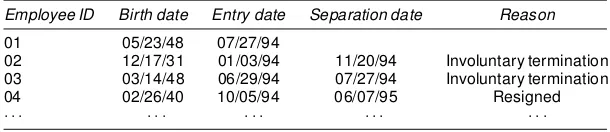
Flow data consist of beginning and ending dates of each em-ployee’s period of employment, that emem-ployee’s birth date, and the reason for separation from employment (if it occurred). We have seen no examples in which employees were rehired for nonoverlapping terms, but such cases could easily be handled by entering one data record for each distinct period of employ-ment. Table 1 is a fragment of a dataset gathered in a hypothet-ical age discrimination case. Data were obtained on all persons employed by the rm any time between 01/01/94 and 01/31/96. Entry Date is the later of 01/03/1994 or the date of hire. The rst record is right censored; that is, that employee was still in the workforce as of 1/31/96, and we are consequently unable to determine the time or cause of his or her eventual separation from the rm (involuntary termination, death, retirement, etc.). The plaintiff obtains such data from the employer in the pre-trial discovery phase. It is generally necessary for the plaintiff’s attorney to justify the need for obtaining data over a particu-lar time period—for example, it might be the period from the imposition of a particular policy to the end of the plaintiff’s employment. Frequently the defendant can convince the court to narrow the scope of the data provided, arguing, for example, that retrieving records more than 5 years old or linking records involving employee transfers between divisions would be bur-densome.
In many litigated cases the observation period is short and corresponds to one large-scale reduction in force (RIF) in which a substantial number of employees were terminated in a com-paratively short period. Kadane (1990) discussed such a case involving four massive ring waves. Data of this sort can be treated as an analysis of the odds ratios (odds on termination of protected versus unprotected employees) in a small number of two-by-two contingency tables. Kadane considered two models for the prior distribution of the odds ratios. In the homogeneous,
Table 1. Flow Data for the Period January 1, 1994 to December 31, 1996
Employee ID Birth date Entry date Separation date Reason
01 05/23/48 07/27/94
02 12/17/31 01/03/94 11/20/94 Involuntary termination 03 03/14/48 06/29/94 07/27/94 Involuntary termination
04 02/26/40 10/05/94 06/07/95 Resigned
¢ ¢ ¢ ¢ ¢ ¢ ¢ ¢ ¢ ¢ ¢ ¢ ¢ ¢ ¢
common odds ratio model, he gave the log odds ratio,¯, a nor-mal distribution with zero mean and xed precision. He com-puted the posterior probability of adverse impact (¯ >0/of the employer’s policy on the protected class for various values of the prior precision. For the inhomogeneous odds ratio model, he assumed independent distributions for the log odds ratios for the four waves of terminations and computed the probability of adverse impact separately for each wave.
This article is an attempt to tackle the analysis of termina-tions occurring at a comparatively low rate, perhaps one or two employees at a time, over a long time period. The problem with this sort of situation is that the disaggregated data consist of numerous two-by-two tables, each involving a small number of terminations but any aggregation of the data (quarterly, semi-annually, etc.) into more substantial two-by-two tables is arbi-trary and somewhat distorts the numbers at risk because some employees will not have been in the workforce for the entire period represented by a given aggregated table. A second, and more important issue is how to deal with the possibility of in-homogeneous odds ratios.
Finkelstein and Levin (1994) suggested that proportional hazards (Cox regression) models could be used to deal with disaggregated employment decisions; however, they assumed a constant log odds ratio over the observation period. We like their idea and in this article show how to allow for the possibil-ity that the relative risk of termination varies over the observa-tion period.
Cox (1972) considered a group of individuals at risk for a particular type of failure (involuntary termination) for all or part of an observation period. Thejth person enters the risk set at timehj(either the date of hire or the beginning of the
observa-tion period) and leaves the risk set at timeTj either by failure
(involuntary termination) or for other reasons (death, voluntary resignation, reassignment, retirement, or the end of the obser-vation period). The survival functionSj.t/DP.Tj>t/is the
probability that the jth employee is involuntarily terminated sometime after time t. The hazard function,¸j.t/, is the
con-ditional probability that personjis terminated at timet given survival to timet, that is,
¸j.t/D¡
wheresjis the derivative ofSj. Integrating (1) produces
Sj.t/Dexp
The Cox proportional hazards model is
¸j.t/D¸.t/exp
observable, time-varying characteristic of the jth person; and
¯.t/is the unobserved, continuous, time-varying log-relative hazard. In our applicationzj.t/D1.0/if personjis (is not)
pro-tected, that is, is (is not) aged 40 or older at timet, and¯ .t/is the logarithm of the odds ratio at timet. The parameter¯ .t/is the instantaneous log odds ratio:
¯ .t/D lim
the number of individuals who were in the workforce at any time during the observation period, andcjD0 if thejth
em-ployee was terminated at timeTjandcjD1 if the employee left
the workforce for some other reason. The likelihood function is
l.¸; ¯jData/D
In practice, times are not recorded continuously, so let us rescale the observation period to the interval [0;1] and assume that time is measured on a nite grid, 0Dt0<t1<¢ ¢ ¢<tpD1.
A sufciently ne grid is dened by the times at which some-thing happened (someone was hired, or left the workforce, or reached age 40). The data are reduced to Ni and ni, the
numbers of employees and protected employees at timeti¡1,
andkiandxi, the numbers of employees and protected
employ-ees involuntarily terminated in the interval.ti¡1;ti]. For data
recorded at this resolution, the likelihood is
l.¸; ¯/D The likelihood depends on the log odds ratio function and the cumulative base rate function only through a nite number of values,¯D.¯1; : : : ; ¯p/0and3D.31; : : : ; 3p/0.
2.1 Hierarchical Priors for Time-Varying Coefcients
Sargent (1997) provided an excellent review of penalized likelihood approaches to modeling time-varying coefcients in proportional hazards models. He argued that these are equivalent to Bayes methods with improper prior distributions on ¯.¢/ and proposed a “exible” model with independent rst differences ¯.tiC1/D¯.ti/CuiC1, where the
innova-tionsuiC1are mutually independent, normal random variables
with mean 0 and precision¿=dtiC1anddtiC1DtiC1¡ti. Under
this model¯ .t/is nowhere smooth—policy, in effect, changes abruptly at every instant. However, in the employment context, we expect changes to be gradual and smooth in the absence of identiable causes such as a change in top management. For that reason we propose a smoothness prior for the log odds ratio,¯ .t/. The smooth model that we describe later is an inte-grated Wiener process with linear drift. Lin and Zhang (1998) used this prior for their generalized additive mixed models; however, their quasi-likelihood approach based on the Laplace approximationappears to fail for employment decision analyses when, for one or more time bins, all or none of the involuntary terminations are in the protected class.
2.2 Smoothness Priors
Let ¯ .t/be a Gaussian process, let ¯iD¯ .ti/, 0·ti·1,
1·i·M, and dene¯D.¯1; : : : ; ¯M/. Specifying a
“smooth-ness” prior requires that we have an opinion about the second derivative of¯ .t/ (see Gersch 1982 and the references cited there). To this end we use the integrated Wiener process rep-resentation (Wahba 1978):
whereW.¢/is a standard Wiener process on the unit interval,
¿ (the precision or “smoothness” parameter) has a proper prior distribution, and the initial state.¯0; ¯00/has a proper prior
dis-tribution independent ofW.¢/and¿. Integrating by parts, we obtain the equivalent representation:
BecausedW.s/is Gaussian white noise, the conditional covari-ance function of¯.¢/is
2.3 Forming an Opinion About Smoothness
The remaining task in specifying the prior distribution of the log odds ratio is to specify prior distributions for the initial state .¯0; ¯00/ and for the smoothness parameter,¿. We have
found that the posterior distribution of¯ .¢/is not sensitive to the prior distribution of the initial state, so we give the initial state a diffuse but proper bivariate normal distribution. How-ever, the smoothness parameter¿ requires more care.
As ¿ ! 1, the Wiener process part of (7) disappears, so this would express certainty that¯ .¢/is exactly linear in time. As ¿ !0, the variance of the¯ .¢/around the linear-in-time mean goes to1, so a good point estimate of¯ .¢/would go through each of the sample points exactly, which offers no smoothness at all. It should come as no surprise, then, that what is essential about a prior on¿ is not to allow too much proba-bility close to 0. In the employment discrimination context, in the examples we have studied the data do not carry much mation about smoothness and it is necessary to have an infor-mative opinion about this parameter. In eliciting opinions about how fast an odds ratio might change, we nd it easiest to think about what might happen during a business quarter. We will use as a reference the prior distribution of a person who thinks that, absent any change in business conditions or management turnover, there is a small probability that the odds of terminat-ing a protected employee relative to an unprotected employee would change more than 15% in a single quarter. For example, if at the beginning of a quarter a protected employee is 5% more
likely to be terminated than an unprotected employee, it would be surprising to see a 20% disparity at the beginning of the next quarter. Our purpose here is to demonstrate a way to develop a reference prior distribution consistent with easily stated as-sumptions. When such analyses are used in litigation, it will be important for the expert to be able to state that his or her con-clusions are robust over a wide range of prior opinions, which is true in the rst case (Case K) that we present but is not in the second case (Case W).
To see what the “no more than 15% change per quar-ter” assumption implies about the prior distribution of the smoothness parameter, consider the central second difference
100D¯ .tCd/¡2¯.t/C¯.t¡d/, where d represents a half-quarter expressed in rescaled time (i.e., as a fraction of the to-tal observation interval). From the covariance function (8), it is easy to compute, variance.100/D2d3=3¿. It is easy to see that if¯ changes by at most .15 over the interval.t¡d;tCd/, thenj100j ·:30. Because we regard values larger than this to be improbably a priori, we can treat .30 as roughly two standard deviations of100. Thus, the prior distribution of¿should place
high probability on the event 2d3=3¿ < :152, that is, 30d3< ¿. Thus, for example, if the observation period is about 16 quar-ters, then a rescaled half-quarter is dD1=32. So the prior distribution should place high probability on the event, ¿ >
30=323¼:0005. A gamma distribution with mean .005 and shape 1 places about 90% of its mass above .0005.
The important thing about a prior on¿is where it puts most of its weight. We believe that other choices of the underlying den-sity would not change the conclusions much. However, shifts in the mean are important, because such shifts control how much smoothing is done. Hence, we study sensitivity mainly by vary-ing the mean, holdvary-ing the rest of the distributional specication unchanged.
2.4 Posterior Distribution
Employers have an absolute right to terminate employees; what they do not have is the right to discriminate on the ba-sis of age without a legitimate business reason unrelated to age. Thus, the base rate is irrelevant to litigation, and we be-lieve that a neutral analyst should give it a exible, diffuse but proper prior distribution. For convenience, we have cho-sen to use a gamma process prior with shape parameter ®
and scale parameter®°. In other words, disjoint increments
3iD3.ti/¡3.ti¡1/DRtti
i¡1¸.t/dt are independent and have
gamma distributions with shape parameter®.ti¡ti¡1/D®dti
and scale parameter®°. The hyperparameters® and° have diffuse but proper log-normal distributions. Consequently, the posterior distribution is proportional to
l.¯; 3/p.¯j¯0; ¯00; ¿ /p.¯0; ¯00/p.¿ /p.3j®; ° /: (9)
The goal is to compute the posterior marginal distribu-tions of the log odds ratios ¯i, 1·i·p, in particular, to
compute the probability that the employer’s policy discrimi-nated against members of the protected class at time ti; that
is,P.¯i>0jData/,
Closed-form integration in (10) is not feasible. Owing to the high dimensionality of the parameter space, numerical quadra-ture is out of the question and the Laplace approximation (Kass, Tierney, and Kadane 1988) would require the maximization of a function over hundreds of arguments. For these reasons we chose to approximate moments and tail areas of the posterior distribution by Markov chain Monte Carlo (MCMC) methods (Tierney 1994; Gelman, Carlin, Stern, and Rubin 1995).
MCMC works by generating a vector-valued Markov chain that has the posterior distribution of the parameter vector as its stationary distribution. An algorithm that generates such a Markov chain is colloquially called asampler. Letµ denote the parameter vector, letf.µjdata/denote the posterior distribution, and letµ1; : : : ; µM be successive realizations ofµ generated by
the sampler. The ergodic theorem (a weak law of large numbers for Markov chains) implies that
1
to be the indicator function of an event such as¯15>0, then
the ergodic theorem states that the relative frequency of that event in the sequenceµ1; : : : ; µM is a consistent estimate of the
posterior probability of that event. However, if the successive realizations generated by the sampler are highly correlated, then the relative frequency may approach the limit very slowly; in this situation the Markov chain is said to “mix” slowly.
In our initial attempts to apply MCMC, we found that the Markov chain did mix very slowly, probably because of the highly collinear covariance matrix of the ¯ vector. We were able to reduce the collinearity, with a resulting improvement in the rate of convergence of the Markov chain, by reexpressing¯ as a linear combination of the initial state vector and the domi-nant principal components of the integrated Wiener process.
2.5 Reexpressing¯
The conditional prior distribution of¯is
p.¯j¯0; ¯00; ¿ /DNp
where the matrixVdepends only on the observation times,
vi;jD whereUis the orthonormal eigenvector matrix andwis the vec-tor of eigenvalues. Suppose that the rstreigenvalues account for, say, 1¡"2of the total variance and letTDUrdiag.pwr/ and zDdiag.w¡:5
r /U0r.¯ ¡ ¹¯/p¿, where Ur is the rst
rcolumns ofUandwris the rstrcomponents ofw. Clearly, the components ofzare iid standard normal and
E£k¿ .¯¡¹¯/¡Tzk2¤D"2E£k¿ .¯¡¹¯/k2¤:
The data in two of these examples come from cases we were involved in—we call them Case K and Case W. In each case one or more plaintiffs were suing a former employer for age discrimination in his or her dismissal. Data for these cases are available in StatLib (Kadane and Woodworth 2001). The third example is a reanalysis of a class action against the U. S. Postal Service (USPS) reported in Freidlin and Gastwirth (2000). All three cases were analyzed via WinBUGS 1.3 (Spiegelhalter, Thomas, and Best 2000). For Cases K and W we used the prin-cipal component representation (12).
3.1 Case K
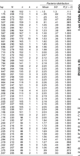
In this case ow data for all individuals employed by the de-fendant at any time during a 1,557-day period (about 17 quar-ters) were available to the statistical expert. During that period 96 employees were involuntarily terminated, 79 of whom were age 40 or above at the time of termination. The data were ag-gregated into 288 time intervals, or bins, bounded by times at which one or more employees entered the workforce, left the workforce, or reached a 40th birthday. The median bin width was 4 days, the mean was about 5 days, and the maximum was 24 days. Based on the discussion in Section 3.2, we prefer that the prior distribution for the smoothness parameter place most of its mass above .0007, so we selected a gamma prior with shape parameter 1 and mean .007; the other parameters were given diffuse but proper priors. Table 2 shows the data, mean, standard deviation, and positive tail area of the log odds ratios for bins with one or more involuntary terminations.
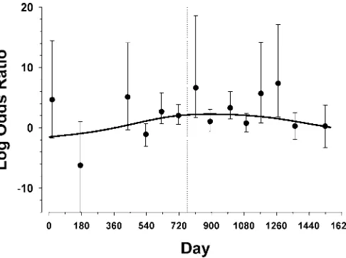
In Figure 1 we show how the smooth model ts the un-smoothed underlying data. To do this, we grouped cases by quarters and computed 95% equal-tail posterior-density cred-ible intervals for the log odds assuming a normal prior with mean 0 and standard deviation 8. We like a standard deviation of 8 for this sort of descriptive display because it is fairly diffuse (there is, for example, 16% prior probability that the odds ratio
Figure 1. Case K: Posterior Mean and Probability of Discrimination for Our Preferred Prior Distribution of the Smoothness Parameter. Ver-tical bars are 95% posterior highest density regions for quarterly ag-gregates with iid N(0, 64) priors. Vertical dotted line indicates date of plaintiff’s dismissal.
Table 2. Data and Posterior Marginal Distributions of the Log Odds Ratio for Case K
Posterior distribution
Day N n k x Mean SD P(¯ >0)
3 190 102 1 1 ¡1.5 1.3 .111
175 208 110 1 0 ¡.95 .82 .110
406 273 150 1 1 .25 .51 .702
444 273 151 1 1 .50 .47 .858
507 283 159 1 0 .91 .41 .985
528 283 159 2 1 1.05 .39 .994
535 284 161 1 1 1.10 .39 .997
555 286 164 1 0 1.23 .38 .999
567 289 167 1 0 1.30 .37 1.000
582 287 167 1 1 1.40 .36 1.000
605 293 170 10 9 1.53 .36 1.000
661 290 165 1 1 1.82 .35 1.000
668 290 165 1 1 1.85 .35 1.000
696 287 163 9 8 1.96 .35 1.000
703 278 155 4 3 1.98 .35 1.000
710 276 152 1 1 2.00 .35 1.000
731 272 150 1 1 2.07 .35 1.000
752 270 147 2 2 2.12 .35 1.000
766 269 143 1 1 2.15 .35 1.000
784 269 141 1 1 2.18 .35 1.000
797 266 138 2 2 2.20 .35 1.000
846 264 136 1 1 2.25 .35 1.000
847 263 135 2 2 2.25 .35 1.000
850 261 133 3 3 2.25 .35 1.000
857 258 130 4 4 2.25 .35 1.000
863 245 120 1 1 2.25 .35 1.000
864 244 119 1 0 2.26 .35 1.000
927 247 121 1 0 2.25 .35 1.000
955 245 120 1 1 2.24 .35 1.000
980 242 118 4 4 2.23 .35 1.000
1,008 236 113 3 3 2.20 .35 1.000
1,017 234 111 1 0 2.19 .35 1.000
1,018 233 111 5 5 2.19 .35 1.000
1,025 227 105 1 1 2.18 .35 1.000
1,037 227 105 1 1 2.16 .35 1.000
1,095 230 105 1 1 2.05 .36 1.000
1,102 226 101 2 1 2.04 .36 1.000
1,106 224 101 1 1 2.03 .36 1.000
1,113 223 100 3 2 2.01 .36 1.000
1,116 220 98 1 0 2.00 .36 1.000
1,141 220 97 1 1 1.94 .36 1.000
1,200 217 93 1 1 1.77 .38 1.000
1,214 216 91 1 1 1.72 .38 1.000
1,224 215 90 2 2 1.69 .39 1.000
1,225 213 88 1 1 1.69 .39 1.000
1,253 215 89 1 1 1.58 .40 1.000
1,256 214 88 1 1 1.56 .40 1.000
1,284 213 89 1 1 1.44 .41 1.000
1,319 210 89 1 1 1.27 .44 .998
1,322 207 88 1 0 1.26 .44 .997
1,361 207 89 1 0 1.06 .48 .982
1,375 204 89 1 1 .99 .50 .972
1,557 205 90 2 1 .09 .93 .568
NOTE: Data and posterior distributions for bins with one or more involuntary terminations. Nworkforce;n, protected;k, involuntary terminations;x, involuntary terminations of pro-tected employees. The smoothness parameter,¿, had a Gamma(1) prior distribution with mean .007, as described in the text. Two chains were run with 50,000 replications each, dis-carding the rst 4,000. The Gelman–Rubin statistic indicated that the chains had converged.
exceeds 3,000) yet prevents innite credible intervals when one category or the other has no terminations. Because this prior pulls the posterior distribution toward 0, it would be difcult for the respondent (the rm) to argue that it is biased in favor of the plaintiff.
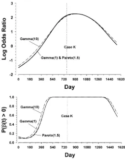
Sensitivity to the prior mean of the smoothness parameter is explored in Figure 2, and sensitivity to the shape of the prior distribution of the smoothness parameter is explored in Fig-ure 3. Between days 528 and 1,322 the probability of
discrim-Figure 2. Case K: Effect of Varying the Prior Mean of the Smooth-ness Parameter (all distributions are Gamma with shape parameter 1).
inationP.¯.t/ >0jdata/exceeds .99 and is insensitive to the prior distribution of the smoothness parameter. The plaintiff in Case K had been dismissed within that interval at day 766. It is not surprising that greater sensitivity to the smoothness para-meter is shown at the start and the end of the period. Thus, if the date of termination of the plaintiff is near the start or the end of the observation period, the conclusionswill be more sensitive to how much smoothing is assumed. This suggests the desirability of designing data collection so that it includes a period of time surrounding the event or events in question.
In addition, we analyzed Case K with Sargent’s (1997) rst-difference prior. The rst-rst-difference prior models the log odds ratio as a linear function plus a Wiener process with preci-sion¿. Thus, the log odds ratio is continuous but not smooth. To scale the prior distribution of the precision of the log odds ratio, we again argue from our prior opinion that the log odds ratio is unlikely to change more than 15% within a quarter. We interpret this as two standard deviations of the rst differ-ence,¯.tCd/¡¯ .t/. The variance of a one-quarter rst dif-ference isd=¿, whered¼1=19 is one quarter expressed as a fraction of the total observation period. Thus, 2pd=¿ ·:15, which implies that the prior should place most of its mass on¿¸9:4. A gamma prior with mean 100 and shape 1 places about 90% of its mass above 9.5. Figure 4 compares the pos-terior mean log odds ratio for Sargent’s smooth model and our continuous model. We found that the posterior distribution for Sargent’s model was not sensitive to the prior means of¿ be-tween 1 and 100.
Figure 3. Case K: Effect of Varying the Shape of the Prior Distribution of the Smoothness Parameter (all distributions have mean .007 and the indicated shape parameters).
We conducted what we believe would be an acceptable fre-quentist analysis via proportional hazards regression to model the time to involuntary termination. The initial model included design variables for membership in the protected group and for the linear interaction of this variable with time. The linear in-teraction was insignicant, so we presume that a frequentist would opt for a constant odds model. The maximum likelihood
Figure 4. Case K: Posterior Mean for Continuous (Wiener process, prior mean smoothness, 100) and Smooth (integrated Wiener process, prior mean smoothness, .007) Distributions of the Log Odds Ratio.
Table 3. Sensitivity Analysisafor Case K
Posterior distribution for Case K
Model Priorb Mean SD P(¯ >0=Data)
Smooth E(¿)D:001 2.22 .37 1.0000 E(¿)D:007
Gamma(1) 2.15 .35 1.0000 Gamma(10) 2.10 .33 1.0000 Pareto(1.5) 2.13 .35 1.0000 E(¿)D:07 2.06 .37 1.0000 E(¿)D100 1.46 .28 1.0000 Continuous E(¿)D100c 2.11 .49 1.0000
Maximum Linear 1.44 .28 n=a
likelihoodd log odds ratio
Constant 1.51 .27 n=a
log odds ratio
aP(¯ >0) for Case K (day 766) is robust to specication of the prior distribution of the
log odds ratio.
bWhere not indicated otherwise, the smoothness parameter,¿, had a Gamma(1) prior with the indicated mean.
cThe shape parameter was 1 except for the smooth prior with mean 100, which had shape parameter 5.
dMaximum likelihood estimates were computed by proportional hazards regression; asymptotic approximations to the one-sidedpvalues are less than .0005.
estimate (and asymptotic standard error) of the log odds ratio is 1.51 (.27), which approximates the posterior mean and stan-dard deviation of this parameter for large values of the smooth-ness parameter (see Table 3).
Although the frequentist and Bayesian analyses reach the same conclusion regarding the presence of discrimination in Case K, we believe that the frequentist analysis does not pro-duce probability statements relevant to the particular case in litigation and in no way constitutes a gold standard for our analysis. On the bases of these analyses, a statistical expert would be able to report that there is strong, robust evidence that discrimination against employees aged 40 and above was present in terminations between days 528 and 1,322 and, in par-ticular, on the day of the plaintiff’s termination.
3.2 Case W
Two plaintiffs, terminated about a year apart, brought sepa-rate age discrimination suits against the employer. The plain-tiffs’ attorneys requested data on all individuals who were in the defendant’s workforce at any time during an approximately 4.5-year observation period containing the termination dates of the plaintiffs. Dates of hire and separation and reason for sepa-ration were provided by the employer as well as age in years at entry into the dataset (the rst day of the observation period or the date of hire) and at separation. The data request was made before the expert statistician was retained and it failed to ask for dates of birth; however, from the ages at entry and exit, it was possible to determine a range of possible birth dates for each employee. Thus, at any given time during the observation period, there is some uncertainty about whether the handful of nonterminated employees near the protected age (40 and older) were or were not in the protected class. We did not attempt to incorporate that uncertainty into this analysis and resolved am-biguities by assuming the birth date was at the center of the interval of dates consistent with the reported ages.
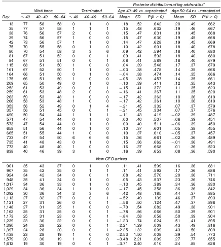
Over an observation period of about 1,600 days, the work-force was reduced by about two-thirds; 103 employees were in-voluntarily terminated in the process. A new CEO took over at
day 862, near the middle of the observation period. The plain-tiffs asserted that employees aged 50 (or 60) and above were targeted for termination under the inuence of the new CEO. So in our reanalysis we have divided the protected class into two subclasses: ages 40–49 and ages 50–64 and estimated sep-arate log odds ratios for each of the protected subclasses rela-tive to the unprotected class. Here we present a fully Bayesian analysis of two models, one with smoothly time-varying odds ratios for each protected subclass and one with smoothly time-varying odds ratios in two phases—before and after the arrival of the new CEO.
The personnel data were aggregated by status (involuntarily terminated, other) into 171 time bins as described in Case K and three age categories (< 40, 40–49, 50–64). Aggregated data
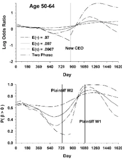
along with posterior means, standard deviations, and proba-bilities of discrimination for the two protected subclasses for bins containing at least one termination are reported in Ta-ble 4. TaTa-ble 4 also reports posterior means, standard deviations, and probabilities of discrimination for our preferred choice of the prior distribution of the smoothness parameters—gamma with shape parameter 1 and mean .007. Figure 5 shows pos-terior means and probabilities of discrimination for different choices of the prior mean of the smoothness parameter. Figure 6 contrasts two-phase and noninterrupted models for employees aged 50–64.
The gures make it clear that the log odds ratios for ei-ther protected subclass were close to 0 before the new CEO arrived. After his arrival it appears that terminations of
em-Table 4. Aggregated Flow Data and Posterior Distributions for Case W
Posterior distributions of log odds ratios¤ Workforce Terminated Age 40–49 vs. unprotected Age 50–64 vs. unprotected Day <40 40–49 50–64 <40 40–49 50–64 Mean SD P(¯ >0) Mean SD P(¯ >0)
13 77 58 58 0 1 0 .18 .52 .642 .20 .49 .662
35 77 57 58 1 1 1 .15 .48 .632 .19 .46 .667
38 76 56 57 2 0 0 .15 .47 .631 .19 .45 .668
39 74 56 57 1 0 0 .15 .47 .630 .19 .45 .668
42 73 56 57 1 1 0 .14 .47 .628 .19 .45 .669
75 70 55 58 0 1 0 .10 .42 .601 .18 .40 .678
80 70 54 58 3 3 6 .09 .42 .594 .18 .40 .680
81 67 51 52 0 0 1 .09 .41 .593 .18 .40 .680
84 67 51 51 0 0 1 .08 .41 .589 .18 .40 .679
115 68 51 50 1 0 0 .04 .39 .548 .17 .37 .679
161 67 52 50 1 1 0 ¡.03 .38 .478 .14 .35 .666
164 66 51 50 0 1 0 ¡.04 .38 .474 .14 .35 .666
175 66 51 50 1 0 0 ¡.05 .38 .457 .14 .35 .661
209 65 50 49 0 1 0 ¡.10 .39 .411 .12 .35 .643
252 61 53 49 0 0 1 ¡.15 .41 .372 .11 .35 .623
259 61 53 48 2 0 0 ¡.16 .41 .367 .11 .35 .620
263 59 53 48 1 0 0 ¡.17 .42 .363 .10 .36 .619
266 58 53 48 1 0 0 ¡.17 .42 .361 .10 .36 .619
353 56 52 49 0 1 4 ¡.21 .45 .332 .07 .37 .579
357 56 51 45 0 0 1 ¡.21 .45 .334 .07 .37 .576
490 50 54 44 1 1 1 ¡.11 .43 .419 ¡.02 .39 .487
571 47 54 44 0 1 0 .00 .40 .507 ¡.06 .39 .451
573 47 54 44 0 1 0 .00 .40 .511 ¡.06 .39 .450
658 51 56 44 0 1 0 .10 .37 .601 ¡.05 .38 .455
665 51 55 44 1 0 0 .10 .37 .610 ¡.05 .37 .457
733 47 54 50 6 6 6 .15 .36 .661 ¡.02 .36 .489
735 41 48 43 0 1 0 .15 .36 .662 ¡.01 .36 .491
773 40 48 40 1 0 0 .16 .37 .668 .01 .36 .523
838 40 46 39 3 1 0 .16 .39 .653 .08 .36 .590
New CEO arrives
901 35 43 37 0 1 0 .11 .41 .599 .16 .36 .681
907 35 42 35 0 1 1 .11 .41 .592 .17 .36 .688
924 34 42 34 0 0 1 .08 .42 .570 .20 .36 .711
948 35 41 34 0 1 0 .05 .43 .537 .23 .36 .746
1,017 34 36 33 0 1 0 ¡.13 .45 .389 .34 .36 .830
1,029 34 36 34 1 1 0 ¡.17 .45 .358 .36 .36 .842
1,092 30 36 34 3 3 6 ¡.42 .48 .185 .44 .37 .885
1,113 27 32 27 0 0 1 ¡.52 .49 .139 .46 .37 .893
1,121 27 31 26 0 0 1 ¡.56 .50 .124 .47 .37 .896
1,148 27 31 25 1 0 0 ¡.70 .54 .082 .49 .38 .901
1,162 25 31 25 0 0 1 ¡.78 .56 .066 .50 .39 .901
1,173 25 31 23 0 0 1 ¡.84 .58 .058 .50 .39 .904
1,239 23 30 22 0 0 1 ¡1.23 .74 .024 .51 .41 .895
1,390 24 28 22 0 0 1 ¡2.21 1.29 .009 .43 .49 .816
1,397 24 28 20 0 0 1 ¡2.25 1.32 .009 .43 .50 .809
1,438 23 28 19 1 0 0 ¡2.53 1.50 .008 .39 .54 .773
1,579 20 30 19 1 0 0 ¡3.48 2.21 .009 .27 .77 .655
1,612 19 30 19 0 0 1 ¡3.71 2.40 .010 .24 .85 .628
¤The smoothness parameter had a Gamma(1) prior with mean .007. Computations were via WinBUGS 1.3. There were 25,000 replications of two chains discarding the rst 4,000.
Figure 5. Case W: Sensitivity to the Smoothness Parameter.
ployees aged 40–49 declined and terminations of employees aged 50–64 increased. This is clearest in the interrupted model, but present to some extent in all models for all smoothness pa-rameter values.
Two plaintiffs, indicated by vertical dotted lines in Figures 5 and 6, brought age discrimination suits against the employer. Plaintiff W1, who was between 50 and 59 years of age, was one of 12 employees involuntarily terminated on day 1,092. His theory of the case was that the new CEO had targeted employ-ees aged 50 and above for termination. Under the two-phase model, which corresponds to the plaintiff’s theory of the case, the probability of discrimination at the time of this plaintiff’s termination was close to 1.00. However, the posterior probabil-ity of discrimination in this case is somewhat sensitive to the choice of model and smoothness parameter (Fig. 6).
In the original case the plaintiff’s statistical expert tabulated involuntary termination rates for each calendar quarter and each age decade. He reported that, “[involuntary] separation rates for the [period beginning at day 481] averaged a little above three percent of the workforce per quarter for ages 20–49, but jumped to six and a half percent for ages 50–59. The 50–59 year age group differed signicantly from the 20–39 year age group (signed-rank test,pD:033, one sided).” Our reanalysis is con-sistent with that conclusion (Fig. 6, two-phase model). The plaintiff alleged and the defendant denied that the new CEO had vowed to weed out older employees. The case was settled before trial.
The case of plaintiff W2 went to trial. This 60-year-old plaintiff was one of 18 employees involuntarily terminated on day 733. On that day three of eight employees (37.5%) aged 60
and up were terminated compared to 15 of 136 (11.0%) employ-ees terminated out of all other age groups (one-sided hyperge-ometricpD:0530). Although the plaintiff had been terminated in the quarter prior to the arrival of the new CEO, the plaintiff’s theory was that the new CEO had been seen on site before he assumed ofce and had inuenced personnel policy decisions prior to his ofcial arrival date.
The defense statistician presented several analyses of the quarterly aggregated data involving different subsets of the ob-servation period and different subgroups of protected and un-protected employees. Based on two-sidedpvalues, he reported no signicant differences between any subgroups; however, one-sidedpvalues are more appropriate in age discrimination cases and several of these are “signicant” or nearly so. Ac-cording to his analysis, for the period after the new CEO was hired, employees aged 50–59 were terminated at a signicantly higher rate than employees aged 20–39 (pD:053, one sided) and employees aged 40–49 (pD:050, one sided); for the pe-riod beginning with the new CEO’s second quarter in ofce the one-sidedp values were .039 and .038, respectively. The de-fense expert did not analyze the interval beginning one quar-ter prior to the arrival of the new CEO—the quarquar-ter in which plaintiff W2 was terminated. Thus, the defense expert’s analy-sis generally agrees with the reanalyanaly-sis presented in this article (Fig. 6). The defense expert also reported several discriminant analyses meant to demonstrate that the mean age of involuntar-ily terminated employees was not different from the mean age of the workforce.
Figure 6. Comparison of Noninterrupted and Two-Phase Odds Ra-tio Models. For the two-phase model the prior distribuRa-tions of the four smoothness parameters were gamma with shape 1 and mean .007.
In response to the latter analysis, the plaintiff’s statistician argued that this was accounted for by a high rate of termina-tion of employees in their rst year of service (“short-term em-ployees”) and presented the results of a proportional hazards regression analysis with constant odds ratios over the entire ob-servation period. The model involved design variables for em-ployees in the rst year of service and for emem-ployees aged 50 and above (thus, the reference category was long-term employ-ees under the age of 50). Employemploy-ees in their rst year of ser-vice were terminated at a signicantly higher rate relative to the reference category (odds ratio D2,pD:01, two sided) as were employees aged 50 and older (odds ratio D1:58,pD:03, two sided).
The plaintiff’s theory of the case, as we understand it, had three components: (1) that the new CEO had been seen on site on several occasions in the quarter before he assumed ofce and was presumably an active participant in personnel policy deci-sions prior to his ofcial arrival date, (2) that the CEO had stated his intent to weed out older employees, and (3) that this had an adverse impact on employees aged 60 and above. The pre-ceding proportional hazards analysis and the analysis of the 18 terminations on day 733 (37% of 60-year-olds terminated ver-sus 11% of all other employees) support the disparate impact theory.
The plaintiff had refused the defendant’s offer of a different job at lower pay. The judge instructed the jury that the plain-tiff had a duty under the law to exercise reasonable diligence to minimize his damages and if they found that he had not done so, then they should reduce his damages by the amount he rea-sonably could have avoided if he had sought out or taken ad-vantage of such an opportunity.The jury found that the plaintiff had proven that age was a determining factor for his discharge but that he had failed to mitigate his damages. Therefore, the award was the difference between what he would have earned at his original salary prior to discharge minus the amount he would have earned had he accepted the lower salaried job. The defendant appealed the case, but settled prior to trial of the ap-peal.
Our reanalysis, with time-varying odds ratios, does not sup-port a theory of adverse impact against employees aged 50–64 prior to the arrival of the new CEO; however, the plaintiff’s specic claim was discrimination against employees aged 60 and older and there does seem to be evidence of this at the time of the plaintiff’s termination (one-sided hypergeomet-ricpD:053).
One Sided or Two Sided? Bayesians compute probabili-ties of relevant events, that is,P.¯.t/ >0jdata/, the conditional probability of discrimination at timetgiven the data. Frequen-tists favor two-sidedpvalues (roughly speaking, the conditional probability, given the assumption of no discrimination, of get-ting the data we got plus the probability of getget-ting even more deviant hypothetical data). As Bayesians, we think such prob-abilities are legally irrelevant. Even within the frequentist par-adigm, however, we think that the use of two-sidedp values is wrong in age discrimination cases. We say this because fre-quentist inference claims to control “Type I error,” that is, to control the conditional probability that an “innocent” employer will be found to discriminate. In age discrimination cases the Type I errors can occur on one side only because only protected
employees have the right to sue under the age discrimination act. Type I errors in the “other tail” would be produced by ev-idence of discrimination against the unprotected class but the unprotected class has no legal right to relief.
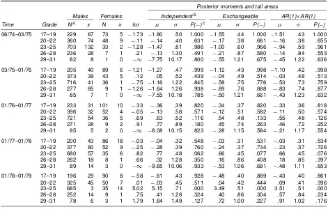
3.3 Valentino v. United States Postal Service
Freidlin and Gastwirth (2000) discussed a case in which the plaintiff led a charge of sex discrimination in promotion at the U.S. Postal Service after she was denied a promotion in mid-1976. The judge certied the women employed at grade 17 and higher as a class. The underlying data, raw log odds ratios, and posterior distributions of the log odds ratios for three dif-ferent specications of the prior are shown in Table 5.
Using frequentist methods, Freidlin and Gastwirth (2000) reported that the p value for discrimination against women was .0006 in period 06/74–03/75, .020 in period 03/75–01/76, and greater than .5 in subsequent periods. The authors advo-cated using CUSUM methods “...to determine the time period when the pattern [of discrimination] remained the same. If the original complaint was led during a period of statistically sig-nicant [discrimination] before the change to fair [employment practices] occurred, then the data are consistent with the plain-tiff’s claim.” They reported that their CUSUM tests showed a signicant change in discrimination over time and that this ef-fect was concentrated in grades 17–19 and 23–25. Apparently they argued from the signicant CUSUM and the pattern of p values for individual time periods that there was discrimi-nation in 1974–1975 and 1975–1976 but not later. However, no formal test or estimate of the location of the changepoint was offered, instead, “...the graph of [the CUSUM test statistic against time] helps to identify the time of the change if one ex-ists... .” Thus, what we appear to be offered is a test of inhomo-geneity of the odds ratio over time combined with inspecting a CUSUM graph and a list ofpvalues for individual time periods. We have reanalyzed the data using three specications of the joint prior distribution of promotion probabilities for each pe-riod, grade, and gender. In the completely independent model, each probability has a prior beta.:1; :1/distribution. In the ran-dom effects model, the log odds ratio (female versus male) for each year and grade consists of a year effect, a grade effect, and an interaction. In the exchangeable model, each class of effects (time, grade, interaction) has an exchangeable multivariate nor-mal prior distribution. In the AR(1)£AR(1) model, time and grade effects have multivariate normal priors with AR(1) co-variance structure and the interactions are exchangeable.
Table 5 shows the posterior mean and standard deviation of the log odds ratio and the probability of discrimination (neg-ative log odds ratio) for each year and grade. We agree with Freidlin and Gastwirth that there is strong evidence of dis-crimination against women in grades 17–19 in periods 1974– 1975 and 1975–1976 and against women in grades 23–25 in year 1974–1975 and not much evidence of discrimination elsewhere. However, we do not see the relevance of a for-mal changepoint test. If there is inhomogeneity, then it should be incorporated into the model. Our analysis does this and it shows that not all members of the certied class have equal claims for relief. We believe that a neutral statistician analyz-ing these data would report that the evidence of
Table 5. Aggregated Data and Posterior Distributions for Valentino v. United States Postal Service
Posterior moments and tail areas
Males Females Independentb Exchangeable AR(1)£AR(1) Time Grade Na x N x lor ¹ ¾ P(¡)c ¹ ¾ P(¡) ¹ ¾ P(¡) 06/74–03/75 17–19 229 67 73 5 ¡1.73 ¡1.80 .50 1.000 ¡1.55 .44 1.000 ¡1.51 .43 1.000 20–22 360 74 48 9 ¡.11 ¡.14 .40 .631 ¡.17 .38 .661 ¡.16 .38 .655 23–25 703 132 33 2 ¡1.28 ¡1.47 .81 .986 ¡1.00 .60 .966 ¡.94 .59 .961 26–28 236 28 7 1 .21 ¡.13 1.30 .491 ¡.21 .87 .580 ¡.14 .84 .553 29–31 82 8 1 0 ¡1 ¡7.75 10.17 .800 ¡.55 1.21 .675 ¡.45 1.22 .636 03/75–01/76 17–19 205 40 89 6 ¡1.21 ¡1.27 .47 .999 ¡1.12 .43 .998 ¡1.10 .42 .998
20–22 373 39 43 5 .12 .05 .52 .439 ¡.04 .49 .514 ¡.03 .48 .513
23–25 716 41 36 1 ¡.75 ¡1.16 1.22 .845 ¡.58 .75 .776 ¡.53 .73 .759 26–28 277 85 9 1 ¡1.26 ¡1.64 1.26 .938 ¡.89 .76 .888 ¡.83 .74 .877 29–31 85 7 1 0 ¡1 ¡7.55 10.18 .785 ¡.50 1.21 .661 ¡.43 1.23 .632 01/76–01/77 17–19 233 31 101 10 ¡.33 ¡.36 .39 .820 ¡.34 .37 .820 ¡.33 .36 .818 20–22 396 32 52 4 ¡.05 ¡.13 .58 .571 ¡.12 .51 .582 ¡.11 .50 .574
23–25 721 54 36 5 .69 .63 .52 .116 .54 .48 .133 .55 .48 .126
26–28 271 28 9 2 .91 .77 .89 .180 .45 .74 .263 .46 .72 .252
29–31 85 5 2 0 ¡1 ¡8.08 10.15 .823 ¡.28 1.15 .584 ¡.21 1.17 .554 01/77–01/78 17–19 200 43 86 18 ¡.03 ¡.04 .32 .548 ¡.03 .31 .531 ¡.03 .31 .534 20–22 377 80 52 9 ¡.25 ¡.28 .39 .760 ¡.24 .37 .734 ¡.23 .37 .726
23–25 680 57 35 6 .82 .77 .48 .062 .66 .45 .077 .66 .45 .076
26–28 262 18 8 1 .66 .32 1.28 .350 .16 .86 .408 .18 .85 .397
29–31 89 14 3 0 ¡1 ¡9.65 10.06 .933 ¡.53 1.06 .681 ¡.48 1.11 .653 01/78–01/79 17–19 196 29 90 8 ¡.58 ¡.61 .43 .928 ¡.48 .40 .889 ¡.43 .40 .861
20–22 325 45 50 7 .01 ¡.03 .45 .511 .04 .42 .444 .09 .41 .396
23–25 685 3 35 14 5.02 5.15 .71 .000 3.49 .51 .000 3.51 .51 .000
26–28 252 14 9 1 .75 .41 1.28 .324 .40 .86 .304 .57 .84 .234
29–31 78 6 3 1 1.79 1.64 1.49 .127 .72 1.00 .227 .91 1.02 .176
aNis the number of employees;xis the number promoted.
b Prior models are independent log odds ratios, exchangeable main effects of time and grade, exchangeable interactions, and AR(1) main effects of time and grade and exchangeable interactions.
cP(¡) is the posterior probability that the log odds ratio is negative—that is, women are less likely to be promoted.
tion is not uniform over grades or time periods, but is concen-trated in grades 17–19 and 23–25 in year 1974–1975 and in grades 17–19 in year 1975–1976. We believe that this is pre-cisely the information that the court needs to determine how the award (if any) should be distributed among members of the certied class.
4. DISCUSSION
A standard criticism of Bayesian analyses is that the prior as-sumptions are arbitrary. One response is, “Compared to what?” Bayesian analysis can be explained to a jury in less convoluted ways than frequentist analyses and makes explicit the necessity to think about sensitive assumptions, rather than covering them with a mantle of false objectivity. The assumption of constant odds ratios in particular and the functional form of a model in general are examples of unexamined subjectivity. The Bayesian approach to model specication involves specifying a prior dis-tribution over a more general class of time-varying odds ratio models. The subjective component of model specication re-sides in the prior distribution of the smoothness parameter. To some the need to think carefully about the prior distribution of the smoothness parameter may seem fatally to open the analysis to attack by opposing counsel on the grounds of arbitrariness. To that we respond that the assumption of a constant or (piece-wise) linear odds ratio is not only arbitrary but implausible on its face and that a more realistic analysis has a better chance of prevailing.
ACKNOWLEDGMENTS
The research of Joseph B. Kadane was partially supported by NSF grant DMS-93-03557. We thank Michael Finkelstein, Joseph Gastwirth, Christopher Genovese, Bruce Levin, John Rolph, and Ashish Sanil for their helpful comments on an ear-lier draft. We also thank Kate Cowles for a key insight in specifying the prior distribution of the smoothness parameter. Finally, we thank Caroline Mitchell for her help with the legal aspects of the problem.
[Received December 2001. Revised January 2003.]
REFERENCES
Cox, D. R. (1972), “Regression Models and Life-Tables,”Journal of the Royal Statistical Society, Ser. B, 34, 187–220.
Finkelstein, M. O., and Levin, B. (1994), “Proportional Hazard Models for Age Discrimination Cases,”Jurimetrics Journal, 34, 153–171.
Freidlin, B., and Gastwirth, J. (2000), “Changepoint Tests Designed for the Analysis of Hiring Data Arising in Employment Discrimination Cases,”
Journal of Business & Economic Statistics, 18, 315–322.
Gastwirth, J. (1992), “Employment Discrimination: A Statistician’s Look at Analysis of Disparate Impact Claims,”Law and Inequality: A Journal of Theory and Practice, 11, 151–179.
Gelman, A., Carlin, J. B., Stern, H. S., and Rubin, D. B. (1995),Bayesian Data Analysis, London: Chapman & Hall.
Gersch, W. (1982), “Smoothness Priors,” inEncyclopedia of Statistical Sci-ences, Vol. 8, eds. S. Kotz, N. L. Johnson, and C. B. Read, New York: Wiley, pp. 518–526.
Kadane, J. B. (1990), “A Statistical Analysis of Adverse Impact of Employer Decisions,”Journal of the American Statistical Association, 85, 925–933. Kadane, J., and Mitchell, C. (1998), “Statistics in Proof of Employment
Dis-crimination Cases,” inControversies in Civil Rights: The Civil Rights Act of 1964 in Perspective, ed. B. Grofman, Charlottesville: University of Virginia Press.
Kadane, J., and Woodworth, G. (2001), “Employment Discrimination Data,” available athttp://lib.stat.cmu.edu/datasets/caseK.txtand/caseW.txt.
Kass, R. E., Tierney, L., and Kadane, J. B. (1988), “Asymptotics in Bayesian Computation,” in Bayesian Statistics 3, eds. J. M. Bernardo, M. H. DeGroot, D. V. Lindley, and A. F. M. Smith, Oxford: Oxford Uni-versity Press, pp. 261–278.
Lin, X., and Zhang, D. (1998), “Semiparametric Stochastic Mixed Models for Longitudinal Data,” Journal of the American Statistical Association, 93, 710–719.
Sargent, D. J. (1997), “A Flexible Approach to Time-Varying Coefcients in the Cox Regression Setting,”Lifetime Data Analysis, 3, 13–25.
Spiegelhalter, D., Thomas, A., and Best, N. (2000),WinBUGS Version 1.3 User Manual, London: MRC Biostatistics Unit, available at http://www.mrc-bsu.cam.ac.uk/bugs.
Tierney, L. (1994), “Markov Chains for Exploring Posterior Distributions” (with discussion),The Annals of Statistics, 22, 1701–1762.
Wahba, G. (1978), “Improper Priors, Spline Smoothing and the Problem of Guarding Against Model Errors in Regression,”Journal of the Royal Statis-tical Society, Ser. B, 40, 364–372.