Elementary
Differential
S E V E N T H
E D I T I O NElementary Differential
Equatio ns and Bo undary
Value Pro blems
William E. Boyce
Edward P. Hamilton Professor EmeritusRichard C. DiPrima
formerly Eliza Ricketts Foundation Professor Department of Mathematical Sciences Rensselaer Polytechnic InstituteJo hn Wiley & So ns, Inc .
PRODUCTION EDITOR Ken Santor
COVER DESIGN Michael Jung
INTERIOR DESIGN Fearn Cutter DeVicq DeCumptich ILLUSTRATION COORDINATOR Sigmund Malinowski
This book was set in Times Roman by Eigentype Compositors, and printed and bound by Von Hoffmann Press, Inc. The cover was printed by Phoenix Color Corporation. This book is printed on acid-free paper.
䊊
∞The paper in this book was manufactured by a mill whose forest management programs include sustained yield harvesting of its timberlands. Sustained yield harvesting principles ensure that the numbers of trees cut each year does not exceed the amount of new growth.
Copyright c2001 John Wiley & Sons, Inc. All rights reserved.
No part of this publication may be reproduced, stored in a retrieval system or transmitted in any form or by any means, electronic, mechanical, photocopying, recording, scanning or otherwise, except as permitted under Sections 107 or 108 of the 1976 United States Copyright Act, without either the prior written permission of the Publisher, or authorization through payment of the appropriate per-copy fee to the Copyright Clearance Center, 222 Rosewood Drive, Danvers, MA 01923, (508) 750-8400, fax (508) 750-4470. Requests to the Publisher for permission should be addressed to the Permissions Department, John Wiley & Sons, Inc., 605 Third Avenue, New York, NY 10158-0012, (212) 850-6011, fax (212) 850-6008, E-Mail: [email protected]. Library of Congress Cataloging in Publication Data:
Boyce, William E.
Elementary differential equations and boundary value problems / William E. Boyce, Richard C. DiPrima – 7th ed.
p. cm. Includes index.
ISBN 0-471-31999-6 (cloth : alk. paper)
1. Differential equations. 2. Boundary value problems. I. DiPrima, Richard C. II. Title QA371 .B773 2000
515’.35–dc21 00-023752
To Elsa and Maureen
To Siobhan, James, Richard, Jr., Carolyn, and Ann
And to the next generation:
William E. Boycereceived his B.A. degree in Mathematics from Rhodes College, and his M.S. and Ph.D. degrees in Mathematics from Carnegie-Mellon University. He is a member of the American Mathematical Society, the Mathematical Association of America, and the Society of Industrial and Applied Mathematics. He is currently the Edward P. Hamilton Distinguished Professor Emeritus of Science Education (Department of Mathematical Sciences) at Rensselaer. He is the author of numerous technical papers in boundary value problems and random differential equations and their applications. He is the author of several textbooks including two differential equations texts, and is the coauthor (with M.H. Holmes, J.G. Ecker, and W.L. Siegmann) of a text on using Maple to explore Calculus. He is also coauthor (with R.L. Borrelli and C.S. Coleman) ofDifferential Equations Laboratory Workbook
(Wiley 1992), which received the EDUCOM Best Mathematics Curricular Innovation Award in 1993. Professor Boyce was a member of the NSF-sponsored CODEE (Consortium for Ordinary Differential Equations Experiments) that led to the widely-acclaimedODE Architect. He has also been active in curriculum innovation and reform. Among other things, he was the initiator of the “Computers in Calculus” project at Rensselaer, partially supported by the NSF. In 1991 he received the William H. Wiley Distinguished Faculty Award given by Rensselaer.
P R E F A C E
This edition, like its predecessors, is written from the viewpoint of the applied mathe-matician, whose interest in differential equations may be highly theoretical, intensely practical, or somewhere in between. We have sought to combine a sound and accurate (but not abstract) exposition of the elementary theory of differential equations with considerable material on methods of solution, analysis, and approximation that have proved useful in a wide variety of applications.
The book is written primarily for undergraduate students of mathematics, science, or engineering, who typically take a course on differential equations during their first or second year of study. The main prerequisite for reading the book is a working knowledge of calculus, gained from a normal two- or three-semester course sequence or its equivalent.
A Changing Learning Environment
The environment in which instructors teach, and students learn, differential equations has changed enormously in the past few years and continues to evolve at a rapid pace. Computing equipment of some kind, whether a graphing calculator, a notebook com-puter, or a desktop workstation is available to most students of differential equations. This equipment makes it relatively easy to execute extended numerical calculations, to generate graphical displays of a very high quality, and, in many cases, to carry out complex symbolic manipulations. A high-speed Internet connection offers an enormous range of further possibilities.
The fact that so many students now have these capabilities enables instructors, if they wish, to modify very substantially their presentation of the subject and their expectations of student performance. Not surprisingly, instructors have widely varying opinions as to how a course on differential equations should be taught under these circumstances. Nevertheless, at many colleges and universities courses on differential equations are becoming more visual, more quantitative, more project-oriented, and less formula-centered than in the past.
Mathematical Modeling
The main reason for solving many differential equations is to try to learn something about an underlying physical process that the equation is believed to model. It is basic to the importance of differential equations that even the simplest equations correspond to useful physical models, such as exponential growth and decay, spring-mass systems, or electrical circuits. Gaining an understanding of a complex natural process is usually accomplished by combining or building upon simpler and more basic models. Thus a thorough knowledge of these models, the equations that describe them, and their solutions, is the first and indispensable step toward the solution of more complex and realistic problems.
More difficult problems often require the use of a variety of tools, both analytical and numerical. We believe strongly that pencil and paper methods must be combined with effective use of a computer. Quantitative results and graphs, often produced by a com-puter, serve to illustrate and clarify conclusions that may be obscured by complicated analytical expressions. On the other hand, the implementation of an efficient numerical procedure typically rests on a good deal of preliminary analysis – to determine the qualitative features of the solution as a guide to computation, to investigate limiting or special cases, or to discover which ranges of the variables or parameters may require or merit special attention.
Thus, a student should come to realize that investigating a difficult problem may well require both analysis and computation; that good judgment may be required to determine which tool is best-suited for a particular task; and that results can often be presented in a variety of forms.
A Flexible Approach
To be widely useful a textbook must be adaptable to a variety of instructional strategies. This implies at least two things. First, instructors should have maximum flexibility to choose both the particular topics that they wish to cover and also the order in which they want to cover them. Second, the book should be useful to students having access to a wide range of technological capability.
Prefa ce ix combinations are also possible and have been used effectively with earlier editions of this book.
With respect to technology, we note repeatedly in the text that computers are ex-tremely useful for investigating differential equations and their solutions, and many of the problems are best approached with computational assistance. Nevertheless, the book is adaptable to courses having various levels of computer involvement, ranging from little or none to intensive. The text is independent of any particular hardware platform or software package. More than 450 problems are marked with the symbol䉴 to indicate that we consider them to be technologically intensive. These problems may call for a plot, or for substantial numerical computation, or for extensive symbolic ma-nipulation, or for some combination of these requirements. Naturally, the designation of a problem as technologically intensive is a somewhat subjective judgment, and the 䉴is intended only as a guide. Many of the marked problems can be solved, at least in part, without computational help, and a computer can be used effectively on many of the unmarked problems.
From a student’s point of view, the problems that are assigned as homework and that appear on examinations drive the course. We believe that the most outstanding feature of this book is the number, and above all the variety and range, of the problems that it contains. Many problems are entirely straightforward, but many others are more challenging, and some are fairly open-ended, and can serve as the basis for independent student projects. There are far more problems than any instructor can use in any given course, and this provides instructors with a multitude of possible choices in tailoring their course to meet their own goals and the needs of their students.
One of the choices that an instructor now has to make concerns the role of computing in the course. For instance, many more or less routine problems, such as those requesting the solution of a first or second order initial value problem, are now easy to solve by a computer algebra system. This edition includes quite a few such problems, just as its predecessors did. We do not state in these problems how they should be solved, because we believe that it is up to each instructor to specify whether their students should solve such problems by hand, with computer assistance, or perhaps both ways. Also, there are many problems that call for a graph of the solution. Instructors have the option of specifying whether they want an accurate computer-generated plot or a hand-drawn sketch, or perhaps both.
There are also a great many problems, as well as some examples in the text, that call for conclusions to be drawn about the solution. Sometimes this takes the form of asking for the value of the independent variable at which the solution has a certain property. Other problems ask for the effect of variations in a parameter, or for the determination of a critical value of a parameter at which the solution experiences a substantial change. Such problems are typical of those that arise in the applications of differential equations, and, depending on the goals of the course, an instructor has the option of assigning few or many of these problems.
Supplementary Materials
Three software packages that are widely used in differential equations courses are
Coombes, B. R. Hunt, R. L. Lipsman, J. E. Osborn, and G. J. Stuck, all at the University of Maryland, provide detailed instructions and examples on the use of these software packages for the investigation and analysis of standard topics in the course.
For the first time, this text is available in anInteractive Edition, featuring an eBook version of the text linked to the award-winningODE Architect. The interactive eBook links live elements in each chapter toODE Architect’s powerful, yet easy-to-use, nu-merical differential equations solver and multimedia modules. The eBook provides a highly interactive environment in which students can construct and explore mathemat-ical models using differential equations to investigate both real-world and hypothetmathemat-ical situations. A companion e-workbook that contains additional problems sets, called Explorations, provides background and opportunities for students to extend the ideas contained in each module. A stand-alone version ofODE Architectis also available.
There is a Student Solutions Manual, by Charles W. Haines of Rochester Institute of Technology, that contains detailed solutions to many of the problems in the book. A complete set of solutions, prepared by Josef Torok of Rochester Institute of Technology, is available to instructors via the Wiley website atwww.wiley.com/college/Boyce.
I mportant Changes in the Seventh Edition
Readers who are familiar with the preceding edition will notice a number of mod-ifications, although the general structure remains much the same. The revisions are designed to make the book more readable by students and more usable in a modern basic course on differential equations. Some changes have to do with content; for example, mathematical modeling, the ideas of stability and instability, and numerical approximations via Euler’s method appear much earlier now than in previous editions. Other modifications are primarily organizational in nature. Most of the changes include new examples to illustrate the underlying ideas.
1. The first two sections of Chapter 1 are new and include an immediate introduction to some problems that lead to differential equations and their solutions. These sections also give an early glimpse of mathematical modeling, of direction fields, and of the basic ideas of stability and instability.
2. Chapter 2 now includes a new Section 2.7 on Euler’s method of numerical ap-proximation. Another change is that most of the material on applications has been consolidated into a single section. Finally, the separate section on first order homoge-neous equations has been eliminated and this material has been placed in the problem set on separable equations instead.
3. Section 4.3 on the method of undetermined coefficients for higher order equations has been simplified by using examples rather than giving a general discussion of the method.
Prefa ce xi 5. An example illustrating the instabilities that can be encountered when dealing with stiff equations has been added to Section 8.5.
6. Section 9.2 has been streamlined by considerably shortening the discussion of au-tonomous systems in general and including instead two examples in which trajectories can be found by integrating a single first order equation.
7. There is a new section 10.1 on two-point boundary value problems for ordinary differential equations. This material can then be called on as the method of separation of variables is developed for partial differential equations. There are also some new three-dimensional plots of solutions of the heat conduction equation and of the wave equation.
As the subject matter of differential equations continues to grow, as new technologies become commonplace, as old areas of application are expanded, and as new ones appear on the horizon, the content and viewpoint of courses and their textbooks must also evolve. This is the spirit we have sought to express in this book.
It is a pleasure to offer my grateful appreciation to the many people who have generously assisted in various ways in the creation of this book.
The individuals listed below reviewed the manuscript and provided numerous valu-able suggestions for its improvement:
Steven M. Baer, Arizona State University Deborah Brandon, Carnegie Mellon University Dante DeBlassie, Texas A & M University
Moses Glasner, Pennsylvania State University–University Park David Gurarie, Case Western Reserve University
Don A. Jones, Arizona State University Duk Lee, Indiana Wesleyan University Gary M. Lieberman, Iowa State University George Majda, Ohio State University Rafe Mazzeo, Stanford University Jeff Morgan, Texas A & M University James Rovnyak, University of Virginia L.F. Shampine, Southern Methodist University Stan Stascinsky, Tarrant County College Robert L. Wheeler, Virginia Tech
I am grateful to my friend of long standing, Charles Haines (Rochester Institute of Technology). In the process of revising once again the Student Solutions Manual he checked the solutions to a great many problems and was responsible for numerous corrections and improvements.
I am indebted to my colleagues and students at Rensselaer whose suggestions and reactions through the years have done much to sharpen my knowledge of differential equations as well as my ideas on how to present the subject.
My thanks also go to the editorial and production staff of John Wiley and Sons. They have always been ready to offer assistance and have displayed the highest standards of professionalism.
Ackno w led gm ents xiii Most important, I thank my wife Elsa for many hours spent proofreading and check-ing details, for raischeck-ing and discusscheck-ing questions both mathematical and stylistic, and above all for her unfailing support and encouragement during the revision process. In a very real sense this book is a joint product.
Preface vii
Chapter 1
I ntroduction 1
1.1 Some Basic Mathematical Models; Direction Fields 1
1.2 Solutions of Some Differential Equations 9
1.3 Classification of Differential Equations 17
1.4 Historical Remarks 23
Chapter 2
First Order Differential Equations 29
2.1 Linear Equations with Variable Coefficients 29
2.2 Separable Equations 40
2.3 Modeling with First Order Equations 47
2.4 Differences Between Linear and Nonlinear Equations 64
2.5 Autonomous Equations and Population Dynamics 74
2.6 Exact Equations and Integrating Factors 89
2.7 Numerical Approximations: Euler’s Method 96
2.8 The Existence and Uniqueness Theorem 105
2.9 First Order Difference Equations 115
Chapter 3
Second Order Linear Equations 129
3.1 Homogeneous Equations with Constant Coefficients 129
3.2 Fundamental Solutions of Linear Homogeneous Equations 137
3.3 Linear Independence and the Wronskian 147
3.4 Complex Roots of the Characteristic Equation 153
3.5 Repeated Roots; Reduction of Order 160
3.6 Nonhomogeneous Equations; Method of Undetermined Coefficients 169
3.7 Variation of Parameters 179
3.8 Mechanical and Electrical Vibrations 186
3.9 Forced Vibrations 200
Chapter 4
Higher Order Linear Equations 209
4.1 General Theory ofnth Order Linear Equations 209
4.2 Homogeneous Equations with Constant Coeffients 214
Co ntents xv 4.3 The Method of Undetermined Coefficients 222
4.4 The Method of Variation of Parameters 226
Chapter 5
Series Solutions of Second Order Linear Equations 231
5.1 Review of Power Series 231
5.2 Series Solutions near an Ordinary Point, Part I 238
5.3 Series Solutions near an Ordinary Point, Part II 249
5.4 Regular Singular Points 255
5.5 Euler Equations 260
5.6 Series Solutions near a Regular Singular Point, Part I 267
5.7 Series Solutions near a Regular Singular Point, Part II 272
5.8 Bessel’s Equation 280
Chapter 6
The Laplace Transform 293
6.1 Definition of the Laplace Transform 293
6.2 Solution of Initial Value Problems 299
6.3 Step Functions 310
6.4 Differential Equations with Discontinuous Forcing Functions 317
6.5 Impulse Functions 324
6.6 The Convolution Integral 330
Chapter 7
Systems of First Order Linear Equations 339
7.1 Introduction 339
7.2 Review of Matrices 348
7.3 Systems of Linear Algebraic Equations; Linear Independence, Eigenvalues, Eigenvectors 357
7.4 Basic Theory of Systems of First Order Linear Equations 368
7.5 Homogeneous Linear Systems with Constant Coefficients 373
7.6 Complex Eigenvalues 384
7.7 Fundamental Matrices 393
7.8 Repeated Eigenvalues 401
7.9 Nonhomogeneous Linear Systems 411
Chapter 8
Numerical Methods 419
8.1 The Euler or Tangent Line Method 419
8.3 The Runge–Kutta Method 435
8.4 Multistep Methods 439
8.5 More on Errors; Stability 445
8.6 Systems of First Order Equations 455
Chapter 9
Nonlinear Differential Equations and Stability 459
9.1 The Phase Plane; Linear Systems 459
9.2 Autonomous Systems and Stability 471
9.3 Almost Linear Systems 479
9.4 Competing Species 491
9.5 Predator–Prey Equations 503
9.6 Liapunov’s Second Method 511
9.7 Periodic Solutions and Limit Cycles 521
9.8 Chaos and Strange Attractors; the Lorenz Equations 532
Chapter 10
Partial Differential Equations and Fourier Series 541
10.1 Two-Point Boundary Valve Problems 541
10.2 Fourier Series 547
10.3 The Fourier Convergence Theorem 558
10.4 Even and Odd Functions 564
10.5 Separation of Variables; Heat Conduction in a Rod 573
10.6 Other Heat Conduction Problems 581
10.7 The Wave Equation; Vibrations of an Elastic String 591
10.8 Laplace’s Equation 604
Appendix A. Derivation of the Heat Conduction Equation 614
Appendix B. Derivation of the Wave Equation 617
Chapter 11
Boundary Value Problems and Sturm–Liouville Theory 621
11.1 The Occurrence of Two Point Boundary Value Problems 621
11.2 Sturm–Liouville Boundary Value Problems 629
11.3 Nonhomogeneous Boundary Value Problems 641
11.4 Singular Sturm–Liouville Problems 656
11.5 Further Remarks on the Method of Separation of Variables: A Bessel Series Expansion 663
11.6 Series of Orthogonal Functions: Mean Convergence 669
Answers to Problems 679
C H A P T E R
1
Intro duc tio n
In this chapter we try in several different ways to give perspective to your study of differential equations. First, we use two problems to illustrate some of the basic ideas that we will return to and elaborate upon frequently throughout the remainder of the book. Later, we indicate several ways of classifying equations, in order to provide organizational structure for the book. Finally, we outline some of the major figures and trends in the historical development of the subject. The study of differential equations has attracted the attention of many of the world’s greatest mathematicians during the past three centuries. Nevertheless, it remains a dynamic field of inquiry today, with many interesting open questions.
1.1 Some Basic Mathematical Models; Direction Fields
Before embarking on a serious study of differential equations (for example, by reading this book or major portions of it) you should have some idea of the possible benefits to be gained by doing so. For some students the intrinsic interest of the subject itself is enough motivation, but for most it is the likelihood of important applications to other fields that makes the undertaking worthwhile.
Many of the principles, or laws, underlying the behavior of the natural world are statements or relations involving rates at which things happen. When expressed in mathematical terms the relations are equations and the rates are derivatives. Equations containing derivatives are differential equations. Therefore, to understand and to investigate problems involving the motion of fluids, the flow of current in electric 1
ODE
circuits, the dissipation of heat in solid objects, the propagation and detection of seismic waves, or the increase or decrease of populations, among many others, it is necessary to know something about differential equations.
A differential equation that describes some physical process is often called a math-ematical modelof the process, and many such models are discussed throughout this book. In this section we begin with two models leading to equations that are easy to solve. It is noteworthy that even the simplest differential equations provide useful models of important physical processes.
E X A M P L E
1
A Falling Object
Suppose that an object is falling in the atmosphere near sea level. Formulate a differ-ential equation that describes the motion.
We begin by introducing letters to represent various quantities of possible interest in this problem. The motion takes place during a certain time interval, so let us uset
to denote time. Also, let us usevto represent the velocity of the falling object. The velocity will presumably change with time, so we think ofv as a function oft; in other words,t is the independent variable andvis the dependent variable. The choice of units of measurement is somewhat arbitrary, and there is nothing in the statement of the problem to suggest appropriate units, so we are free to make any choice that seems reasonable. To be specific, let us measure timet in seconds and velocityvin meters/second. Further, we will assume thatvis positive in the downward direction, that is, when the object is falling.
The physical law that governs the motion of objects is Newton’s second law, which states that the mass of the object times its acceleration is equal to the net force on the object. In mathematical terms this law is expressed by the equation
F=ma. (1)
In this equationmis the mass of the object,ais its acceleration, andFis the net force exerted on the object. To keep our units consistent, we will measurem in kilograms,a
in meters/second2, andFin newtons. Of course,ais related tovbya=dv/dt, so we can rewrite Eq. (1) in the form
F =m(dv/dt). (2)
Next, consider the forces that act on the object as it falls. Gravity exerts a force equal to the weight of the object, ormg, wheregis the acceleration due to gravity. In the units we have chosen,ghas been determined experimentally to be approximately equal to 9.8 m/sec2near the earth’s surface. There is also a force due to air resistance, or drag, which is more difficult to model. This is not the place for an extended discussion of the drag force; suffice it to say that it is often assumed that the drag is proportional to the velocity, and we will make that assumption here. Thus the drag force has the magnitudeγ v, whereγ is a constant called the drag coefficient.
In writing an expression for the net forceFwe need to remember that gravity always acts in the downward (positive) direction, while drag acts in the upward (negative) direction, as shown in Figure 1.1.1. Thus
1.1 So m e Ba s ic Ma them a tica l Mo d els ; Directio n Field s 3 and Eq. (2) then becomes
mdv
dt =mg−γ v. (4)
Equation (4) is a mathematical model of an object falling in the atmosphere near sea level. Note that the model contains the three constantsm,g, andγ. The constantsm
andγ depend very much on the particular object that is falling, and usually will be different for different objects. It is common to refer to them as parameters, since they may take on a range of values during the course of an experiment. On the other hand, the value ofgis the same for all objects.
γ υ
mg m
FIGURE 1.1.1 Free-body diagram of the forces on a falling object.
To solve Eq. (4) we need to find a functionv=v(t)that satisfies the equation. It is not hard to do this and we will show you how in the next section. For the present, however, let us see what we can learn about solutions without actually finding any of them. Our task is simplified slightly if we assign numerical values tomandγ, but the procedure is the same regardless of which values we choose. So, let us suppose that
m =10 kg andγ =2 kg/sec. If the units forγ seem peculiar, remember thatγ vmust have the units of force, namely, kg-m/sec2. Then Eq. (4) can be rewritten as
dv
dt =9.8−
v
5. (5)
E X A M P LE
2
A Falling Object (continued)
Investigate the behavior of solutions of Eq. (5) without actually finding the solutions in question.
We will proceed by looking at Eq. (5) from a geometrical viewpoint. Suppose that v has a certain value. Then, by evaluating the right side of Eq. (5), we can find the corresponding value ofdv/dt. For instance, ifv=40, thendv/dt =1.8. This means that the slope of a solutionv=v(t)has the value 1.8 at any point wherev=40. We can display this information graphically in thetv-plane by drawing short line segments, or arrows, with slope 1.8 at several points on the linev=40. Similarly, ifv=50, then
dv/dt = −0.2, so we draw line segments with slope−0.2 at several points on the line v=50. We obtain Figure 1.1.2 by proceeding in the same way with other values of v. Figure 1.1.2 is an example of what is called adirection fieldor sometimes aslope field.
2 4 6 8 10 t 48
44
40 52 60
56
υ
FIGURE 1.1.2 A direction field for Eq. (5).
no graphs of solutions appear in the figure, we can nonetheless draw some qualitative conclusions about the behavior of solutions. For instance, ifv is less than a certain critical value, then all the line segments have positive slopes, and the speed of the falling object increases as it falls. On the other hand, ifvis greater than the critical value, then the line segments have negative slopes, and the falling object slows down as it falls. What is this critical value ofvthat separates objects whose speed is increasing from those whose speed is decreasing? Referring again to Eq. (5), we ask what value ofvwill causedv/dt to be zero? The answer isv=(5)(9.8)=49 m/sec.
In fact, the constant function v(t)=49 is a solution of Eq. (5). To verify this statement, substitutev(t)=49 into Eq. (5) and observe that each side of the equation is zero. Because it does not change with time, the solution v(t)=49 is called an
equilibrium solution. It is the solution that corresponds to a balance between gravity and drag. In Figure 1.1.3 we show the equilibrium solutionv(t)=49 superimposed on the direction field. From this figure we can draw another conclusion, namely, that all other solutions seem to be converging to the equilibrium solution ast increases.
2 4 6 8 10 t
48
44
40 52 60
56
υ
1.1 So m e Ba s ic Ma them a tica l Mo d els ; Directio n Field s 5 The approach illustrated in Example 2 can be applied equally well to the more general Eq. (4), where the parametersm andγ are unspecified positive numbers. The results are essentially identical to those of Example 2. The equilibrium solution of Eq. (4) isv(t)=mg/γ. Solutions below the equilibrium solution increase with time, those above it decrease with time, and all other solutions approach the equilibrium solution astbecomes large.
Direction Fields. Direction fields are valuable tools in studying the solutions of differential equations of the form
d y
dt = f(t,y), (6)
where f is a given function of the two variablest and y, sometimes referred to as therate function. The equation in Example 2 is somewhat simpler in that in it f is a function of the dependent variable alone and not of the independent variable. A useful direction field for equations of the general form (6) can be constructed by evaluating f
at each point of a rectangular grid consisting of at least a few hundred points. Then, at each point of the grid, a short line segment is drawn whose slope is the value of f
at that point. Thus each line segment is tangent to the graph of the solution passing through that point. A direction field drawn on a fairly fine grid gives a good picture of the overall behavior of solutions of a differential equation. The construction of a direction field is often a useful first step in the investigation of a differential equation.
Two observations are worth particular mention. First, in constructing a direction field, we do not have to solve Eq. (6), but merely evaluate the given function f(t,y) many times. Thus direction fields can be readily constructed even for equations that may be quite difficult to solve. Second, repeated evaluation of a given function is a task for which a computer is well suited and you should usually use a computer to draw a direction field. All the direction fields shown in this book, such as the one in Figure 1.1.2, were computer-generated.
Field Mice and Owls. Now let us look at another quite different example. Consider a population of field mice who inhabit a certain rural area. In the absence of predators we assume that the mouse population increases at a rate proportional to the current population. This assumption is not a well-established physical law (as Newton’s law of motion is in Example 1), but it is a common initial hypothesis1in a study of population growth. If we denote time byt and the mouse population by p(t), then the assumption about population growth can be expressed by the equation
d p
dt =r p, (7)
where the proportionality factorr is called therate constantorgrowth rate. To be specific, suppose that time is measured in months and that the rate constantr has the value 0.5/month. Then each term in Eq. (7) has the units of mice/month.
Now let us add to the problem by supposing that several owls live in the same neighborhood and that they kill 15 field mice per day. To incorporate this information
1
into the model, we must add another term to the differential equation (7), so that it becomes
d p
dt =0.5p−450. (8)
Observe that the predation term is−450 rather than−15 because time is measured in months and the monthly predation rate is needed.
E X A M P L E
3
Investigate the solutions of Eq. (8) graphically.
A direction field for Eq. (8) is shown in Figure 1.1.4. For sufficiently large values ofpit can be seen from the figure, or directly from Eq. (8) itself, thatd p/dtis positive, so that solutions increase. On the other hand, for small values of pthe opposite is the case. Again, the critical value ofpthat separates solutions that increase from those that decrease is the value ofpfor whichd p/dt is zero. By settingd p/dt equal to zero in Eq. (8) and then solving forp, we find the equilibrium solution p(t)=900 for which the growth term and the predation term in Eq. (8) are exactly balanced. The equilibrium solution is also shown in Figure 1.1.4.
1 2 3 4 5 t
900
850
800 950 1000 p
FIGURE 1.1.4 A direction field for Eq. (8).
Comparing this example with Example 2, we note that in both cases the equilibrium solution separates increasing from decreasing solutions. However, in Example 2 other solutions converge to, or are attracted by, the equilibrium solution, while in Example 3 other solutions diverge from, or are repelled by, the equilibrium solution. In both cases the equilibrium solution is very important in understanding how solutions of the given differential equation behave.
A more general version of Eq. (8) is
d p
1.1 So m e Ba s ic Ma them a tica l Mo d els ; Directio n Field s 7 where the growth rater and the predation ratekare unspecified. Solutions of this more general equation behave very much like those of Eq. (8). The equilibrium solution of Eq. (9) is p(t)=k/r. Solutions above the equilibrium solution increase, while those below it decrease.
You should keep in mind that both of the models discussed in this section have their limitations. The model (5) of the falling object ceases to be valid as soon as the object hits the ground, or anything else that stops or slows its fall. The population model (8) eventually predicts negative numbers of mice (if p<900) or enormously large numbers (if p>900). Both these predictions are unrealistic, so this model becomes unacceptable after a fairly short time interval.
Constructing Mathematical Models. In applying differential equations to any of the numerous fields in which they are useful, it is necessary first to formulate the appropri-ate differential equation that describes, or models, the problem being investigappropri-ated. In this section we have looked at two examples of this modeling process, one drawn from physics and the other from ecology. In constructing future mathematical models your-self, you should recognize that each problem is different, and that successful modeling is not a skill that can be reduced to the observance of a set of prescribed rules. Indeed, constructing a satisfactory model is sometimes the most difficult part of the problem. Nevertheless, it may be helpful to list some steps that are often part of the process:
1. Identify the independent and dependent variables and assign letters to represent them. The independent variable is often time.
2. Choose the units of measurement for each variable. In a sense the choice of units is arbitrary, but some choices may be much more convenient than others. For example, we chose to measure time in seconds in the falling object problem and in months in the population problem.
3. Articulate the basic principle that underlies or governs the problem you are inves-tigating. This may be a widely recognized physical law, such as Newton’s law of motion, or it may be a more speculative assumption that may be based on your own experience or observations. In any case, this step is likely not to be a purely mathematical one, but will require you to be familiar with the field in which the problem lies.
4. Express the principle or law in step 3 in terms of the variables you chose in step 1. This may be easier said than done. It may require the introduction of physical constants or parameters (such as the drag coefficient in Example 1) and the determination of appropriate values for them. Or it may involve the use of auxiliary or intermediate variables that must then be related to the primary variables.
5. Make sure that each term in your equation has the same physical units. If this is not the case, then your equation is wrong and you should seek to repair it. If the units agree, then your equation at least is dimensionally consistent, although it may have other shortcomings that this test does not reveal.
PROBLEMS
In each of Problems 1 through 6 draw a direction field for the given differential equation. Based on the direction field, determine the behavior ofyast→ ∞. If this behavior depends on the initial value ofyatt=0, describe this dependency.䉴 1. y′=3−2y 䉴 2. y′=2y−3
䉴 3. y′=3+2y 䉴 4. y′= −1−2y
䉴 5. y′=1+2y 䉴 6. y′=y+2
In each of Problems 7 through 10 write down a differential equation of the formd y/dt=ay+b whose solutions have the required behavior ast→ ∞.
7. All solutions approachy=3. 8. All solutions approachy=2/3. 9. All other solutions diverge fromy=2. 10. All other solutions diverge fromy=1/3.
In each of Problems 11 through 14 draw a direction field for the given differential equation. Based on the direction field, determine the behavior ofyast→ ∞. If this behavior depends on the initial value of y att=0, describe this dependency. Note that in these problems the equations are not of the formy′=ay+band the behavior of their solutions is somewhat more complicated than for the equations in the text.
䉴 11. y′=y(4−y) 䉴 12. y′= −y(5−y)
䉴 13. y′=y2 䉴 14. y′=y(y−2)2
15. A pond initially contains 1,000,000 gal of water and an unknown amount of an undesirable chemical. Water containing 0.01 gram of this chemical per gallon flows into the pond at a rate of 300 gal/min. The mixture flows out at the same rate so the amount of water in the pond remains constant. Assume that the chemical is uniformly distributed throughout the pond.
(a) Write a differential equation whose solution is the amount of chemical in the pond at any time.
(b) How much of the chemical will be in the pond after a very long time? Does this limiting amount depend on the amount that was present initially?
16. A spherical raindrop evaporates at a rate proportional to its surface area. Write a differential equation for the volume of the raindrop as a function of time.
17. A certain drug is being administered intravenously to a hospital patient. Fluid containing 5 mg/cm3of the drug enters the patient’s bloodstream at a rate of 100 cm3/hr. The drug is absorbed by body tissues or otherwise leaves the bloodstream at a rate proportional to the amount present, with a rate constant of 0.4 (hr)−1.
(a) Assuming that the drug is always uniformly distributed throughout the bloodstream, write a differential equation for the amount of the drug that is present in the bloodstream at any time.
(b) How much of the drug is present in the bloodstream after a long time?
䉴 18. For small, slowly falling objects the assumption made in the text that the drag force is proportional to the velocity is a good one. For larger, more rapidly falling objects it is more accurate to assume that the drag force is proportional to the square of the velocity.2 (a) Write a differential equation for the velocity of a falling object of massmif the drag force is proportional to the square of the velocity.
(b) Determine the limiting velocity after a long time.
(c) Ifm=10 kg, find the drag coefficient so that the limiting velocity is 49 m /sec. (d) Using the data in part (c), draw a direction field and compare it with Figure 1.1.3.
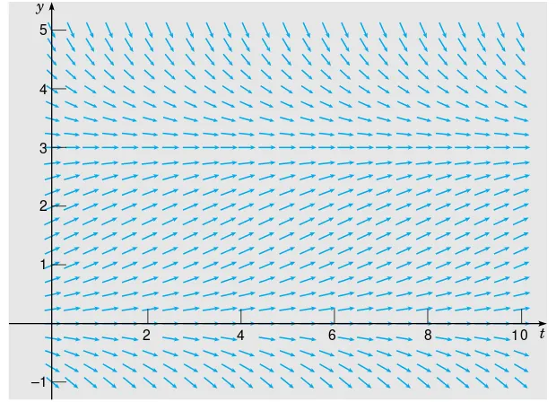
1.2 So lu tio ns o f So m e Differentia l Eq u a tio ns 9 In each of Problems 19 through 26 draw a direction field for the given differential equation. Based on the direction field, determine the behavior of yast→ ∞. If this behavior depends on the initial value of yatt=0, describe this dependency. Note that the right sides of these equations depend ont as well as y; therefore their solutions can exhibit more complicated behavior than those in the text.
䉴 19. y′= −2+t−y 䉴 20. y′=t e−2t−2y
䉴 21. y′=e−t+y 䉴 22. y′=t+2y
䉴 23. y′=3 sint+1+y 䉴 24. y′=2t−1−y2 䉴 25. y′= −(2t+y)/2y 䉴 26. y′=y3/6−y−t2/3
1.2 Solutions of Some Differential Equations
In the preceding section we derived differential equations,
mdv
dt =mg−γ v (1)
and
d p
dt =r p−k, (2)
which model a falling object and a population of field mice preyed upon by owls, respectively. Both these equations are of the general form
d y
dt =ay−b, (3)
whereaandbare given constants. We were able to draw some important qualitative conclusions about the behavior of solutions of Eqs. (1) and (2) by considering the associated direction fields. To answer questions of a quantitative nature, however, we need to find the solutions themselves, and we now investigate how to do that.
E X A M P LE
1
Field Mice and Owls (continued)
Consider the equation
d p
dt =0.5p−450, (4)
which describes the interaction of certain populations of field mice and owls [see Eq. (8) of Section 1.1]. Find solutions of this equation.
To solve Eq. (4) we need to find functions p(t) that, when substituted into the equation, reduce it to an obvious identity. Here is one way to proceed. First, rewrite Eq. (4) in the form
d p
dt =
p−900
2 , (5)
or, if p=900,
d p/dt p−900=
1
2. (6)
Since, by the chain rule, the left side of Eq. (6) is the derivative of ln|p−900| with respect tot, it follows that
d
dt ln|p−900| =
1
2. (7)
Then, by integrating both sides of Eq. (7), we obtain ln|p−900| = t
2+C, (8)
whereC is an arbitrary constant of integration. Therefore, by taking the exponential of both sides of Eq. (8), we find that
|p−900| =eCet/2, (9)
or
p−900= ±eCet/2, (10)
and finally
p=900+cet/2, (11)
wherec= ±eC is also an arbitrary (nonzero) constant. Note that the constant function
p=900 is also a solution of Eq. (5) and that it is contained in the expression (11) if we allowcto take the value zero. Graphs of Eq. (11) for several values ofcare shown in Figure 1.2.1.
900
600
1 2 3 4 5 t
700 800 1000 1100 1200 p
FIGURE 1.2.1 Graphs of Eq. (11) for several values ofc.
Note that they have the character inferred from the direction field in Figure 1.1.4. For instance, solutions lying on either side of the equilibrium solutionp=900 tend to diverge from that solution.
1.2 So lu tio ns o f So m e Differentia l Eq u a tio ns 11 might have. This is typical of what happens when you solve a differential equation. The solution process involves an integration, which brings with it an arbitrary constant, whose possible values generate an infinite family of solutions.
Frequently, we want to focus our attention on a single member of the infinite family of solutions by specifying the value of the arbitrary constant. Most often, we do this indirectly by specifying instead a point that must lie on the graph of the solution. For example, to determine the constantcin Eq. (11), we could require that the population have a given value at a certain time, such as the value 850 at timet =0. In other words, the graph of the solution must pass through the point(0,850). Symbolically, we can express this condition as
p(0)=850. (12)
Then, substitutingt =0 and p=850 into Eq. (11), we obtain 850=900+c.
Hencec= −50, and by inserting this value in Eq. (11), we obtain the desired solution, namely,
p=900−50et/2. (13)
The additional condition (12) that we used to determinecis an example of aninitial condition. The differential equation (4) together with the initial condition (12) form aninitial value problem.
Now consider the more general problem consisting of the differential equation (3)
d y
dt =ay−b
and the initial condition
y(0)= y0, (14)
where y0is an arbitrary initial value. We can solve this problem by the same method as in Example 1. Ifa=0 and y=b/a, then we can rewrite Eq. (3) as
d y/dt
y−(b/a) =a. (15)
By integrating both sides, we find that
ln|y−(b/a)| =at+C, (16)
whereCis arbitrary. Then, taking the exponential of both sides of Eq. (16) and solving fory, we obtain
y =(b/a)+ceat, (17)
where c= ±eC is also arbitrary. Observe thatc=0 corresponds to the equilibrium solution y=b/a. Finally, the initial condition (14) requires thatc= y0−(b/a), so the solution of the initial value problem (3), (14) is
y=(b/a)+[y0−(b/a)]eat. (18)
The expression (17) contains all possible solutions of Eq. (3) and is called the
a particular value ofc, and is the graph of the solution corresponding to that value ofc. Satisfying an initial condition amounts to identifying the integral curve that passes through the given initial point.
To relate the solution (18) to Eq. (2), which models the field mouse population, we need only replaceaby the growth raterandbby the predation ratek. Then the solution (18) becomes
p=(k/r)+[p0−(k/r)]er t, (19) where p0 is the initial population of field mice. The solution (19) confirms the con-clusions reached on the basis of the direction field and Example 1. Ifp0 =k/r, then from Eq. (19) it follows that p=k/r for allt; this is the constant, or equilibrium, solution. If p0=k/r, then the behavior of the solution depends on the sign of the coefficientp0−(k/r)of the exponential term in Eq. (19). If p0 >k/r, then pgrows exponentially with time t; if p0 <k/r, then p decreases and eventually becomes zero, corresponding to extinction of the field mouse population. Negative values ofp, while possible for the expression (19), make no sense in the context of this particular problem.
To put the falling object equation (1) in the form (3), we must identifyawith−γ /m
andbwith−g. Making these substitutions in the solution (18), we obtain
v=(mg/γ )+[v0−(mg/γ )]e−γt/m, (20) wherev0 is the initial velocity. Again, this solution confirms the conclusions reached in Section 1.1 on the basis of a direction field. There is an equilibrium, or constant, solutionv=mg/γ, and all other solutions tend to approach this equilibrium solution. The speed of convergence to the equilibrium solution is determined by the exponent −γ /m. Thus, for a given massmthe velocity approaches the equilibrium value faster as the drag coefficientγ increases.
E X A M P L E
2
A Falling Object (continued)
Suppose that, as in Example 2 of Section 1.1, we consider a falling object of mass
m=10 kg and drag coefficientγ =2 kg/sec. Then the equation of motion (1) becomes
dv
dt =9.8−
v
5. (21)
Suppose this object is dropped from a height of 300 m. Find its velocity at any timet. How long will it take to fall to the ground, and how fast will it be moving at the time of impact?
The first step is to state an appropriate initial condition for Eq. (21). The word “dropped” in the statement of the problem suggests that the initial velocity is zero, so we will use the initial condition
v(0)=0. (22)
The solution of Eq. (21) can be found by substituting the values of the coefficients into the solution (20), but we will proceed instead to solve Eq. (21) directly. First, rewrite the equation as
dv/dt
v−49 = − 1
1.2 So lu tio ns o f So m e Differentia l Eq u a tio ns 13 By integrating both sides we obtain
ln|v−49| = −t
5+C, (24)
and then the general solution of Eq. (21) is
v=49+ce−t/5, (25)
where cis arbitrary. To determinec, we substitutet =0 andv=0 from the initial condition (22) into Eq. (25), with the result thatc= −49. Then the solution of the initial value problem (21), (22) is
v=49(1−e−t/5). (26)
Equation (26) gives the velocity of the falling object at any positive time (before it hits the ground, of course).
Graphs of the solution (25) for several values ofcare shown in Figure 1.2.2, with the solution (26) shown by the heavy curve. It is evident that all solutions tend to approach the equilibrium solutionv=49. This confirms the conclusions we reached in Section 1.1 on the basis of the direction fields in Figures 1.1.2 and 1.1.3.
100
80
60
40
20
2 4 6 8 10 12 t
v
v = 49 (1 – e–t/5)
(10.51, 43.01)
FIGURE 1.2.2 Graphs of the solution (25) for several values ofc.
To find the velocity of the object when it hits the ground, we need to know the time at which impact occurs. In other words, we need to determine how long it takes the object to fall 300 m. To do this, we note that the distance x the object has fallen is related to its velocityvby the equationv=d x/dt, or
d x
dt =49(1−e
−t/5
). (27)
Consequently,
wherec is an arbitrary constant of integration. The object starts to fall whent =0, so we know thatx =0 whent =0. From Eq. (28) it follows thatc= −245, so the distance the object has fallen at timetis given by
x =49t+245e−t/5−245. (29)
LetT be the time at which the object hits the ground; thenx =300 whent =T. By substituting these values in Eq. (29) we obtain the equation
49T +245e−T/5−545=0. (30)
The value ofT satisfying Eq. (30) can be readily approximated by a numerical process using a scientific calculator or computer, with the result thatT ∼=10.51 sec. At this time, the corresponding velocityvT is found from Eq. (26) to bevT ∼=43.01 m/sec.
Further Remarks on Mathematical Modeling. Up to this point we have related our discussion of differential equations to mathematical models of a falling object and of a hypothetical relation between field mice and owls. The derivation of these models may have been plausible, and possibly even convincing, but you should remember that the ultimate test of any mathematical model is whether its predictions agree with observations or experimental results. We have no actual observations or experimental results to use for comparison purposes here, but there are several sources of possible discrepancies.
In the case of the falling object the underlying physical principle (Newton’s law of motion) is well-established and widely applicable. However, the assumption that the drag force is proportional to the velocity is less certain. Even if this assumption is correct, the determination of the drag coefficientγ by direct measurement presents difficulties. Indeed, sometimes one finds the drag coefficient indirectly, for example, by measuring the time of fall from a given height, and then calculating the value ofγ that predicts this time.
The model of the field mouse population is subject to various uncertainties. The determination of the growth rater and the predation ratekdepends on observations of actual populations, which may be subject to considerable variation. The assumption thatr andkare constants may also be questionable. For example, a constant predation rate becomes harder to sustain as the population becomes smaller. Further, the model predicts that a population above the equilibrium value will grow exponentially larger and larger. This seems at variance with the behavior of actual populations; see the further discussion of population dynamics in Section 2.5.
Even if a mathematical model is incomplete or somewhat inaccurate, it may never-theless be useful in explaining qualitative features of the problem under investigation. It may also be valid under some circumstances but not others. Thus you should always use good judgment and common sense in constructing mathematical models and in using their predictions.
PROBLEMS
䉴 1. Solve each of the following initial value problems and plot the solutions for several values of y0. Then describe in a few words how the solutions resemble, and differ from, each other.
1.2 So lu tio ns o f So m e Differentia l Eq u a tio ns 15 䉴 2. Follow the instructions for Problem 1 for the following initial value problems:
(a) d y/dt =y−5, y(0)=y0 (b) d y/dt =2y−5, y(0)=y0 (c) d y/dt =2y−10, y(0)=y0 3. Consider the differential equation
d y/dt= −ay+b,
where bothaandbare positive numbers. (a) Solve the differential equation.
(b) Sketch the solution for several different initial conditions.
(c) Describe how the solutions change under each of the following conditions: i. aincreases.
ii. bincreases.
iii. Bothaandbincrease, but the ratiob/aremains the same. 4. Here is an alternative way to solve the equation
d y/dt =ay−b. (i)
(a) Solve the simpler equation
d y/dt=ay. (ii)
Call the solutiony1(t).
(b) Observe that the only difference between Eqs. (i) and (ii) is the constant−bin Eq. (i). Therefore it may seem reasonable to assume that the solutions of these two equations also differ only by a constant. Test this assumption by trying to find a constantk so that y=y1(t)+kis a solution of Eq. (i).
(c) Compare your solution from part (b) with the solution given in the text in Eq. (17). Note:This method can also be used in some cases in which the constantbis replaced by a functiong(t). It depends on whether you can guess the general form that the solution is likely to take. This method is described in detail in Section 3.6 in connection with second order equations.
5. Use the method of Problem 4 to solve the equation
d y/dt= −ay+b.
6. The field mouse population in Example 1 satisfies the differential equation
d p/dt =0.5p−450.
(a) Find the time at which the population becomes extinct if p(0)=850. (b) Find the time of extinction ifp(0)=p0, where 0<p0<900.
(c) Find the initial populationp0if the population is to become extinct in 1 year. 7. Consider a population p of field mice that grows at a rate proportional to the current
population, so thatd p/dt=r p.
(a) Find the rate constantrif the population doubles in 30 days. (b) Findrif the population doubles inNdays.
8. The falling object in Example 2 satisfies the initial value problem
dv/dt =9.8−(v/5), v(0)=0.
(a) Find the time that must elapse for the object to reach 98% of its limiting velocity. (b) How far does the object fall in the time found in part (a)?
9. Modify Example 2 so that the falling object experiences no air resistance. (a) Write down the modified initial value problem.
10. A radioactive material, such as the isotope thorium-234, disintegrates at a rate proportional to the amount currently present. IfQ(t)is the amount present at timet, thend Q/dt= −r Q, wherer>0 is the decay rate.
(a) If 100 mg of thorium-234 decays to 82.04 mg in 1 week, determine the decay rater. (b) Find an expression for the amount of thorium-234 present at any timet.
(c) Find the time required for the thorium-234 to decay to one-half its original amount. 11. Thehalf-lifeof a radioactive material is the time required for an amount of this material
to decay to one-half its original value. Show that, for any radioactive material that decays according to the equationQ′= −r Q, the half-lifeτand the decay ratersatisfy the equation rτ=ln 2.
12. Radium-226 has a half-life of 1620 years. Find the time period during which a given amount of this material is reduced by one-quarter.
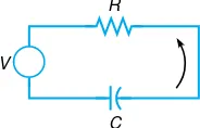
13. Consider an electric circuit containing a capacitor, resistor, and battery; see Figure 1.2.3. The chargeQ(t)on the capacitor satisfies the equation3
Rd Q dt +
Q C =V,
whereRis the resistance,Cis the capacitance, andVis the constant voltage supplied by the battery.
V
R
C
FIGURE 1.2.3 The electric circuit of Problem 13.
(a) IfQ(0)=0, findQ(t)at any timet, and sketch the graph ofQversust. (b) Find the limiting valueQLthatQ(t)approaches after a long time.
(c) Suppose thatQ(t1)=QLand that the battery is removed from the circuit att=t1. FindQ(t)fort>t1and sketch its graph.
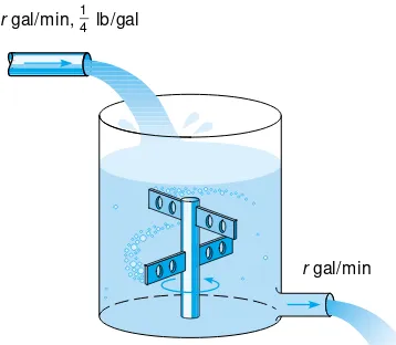
䉴 14. A pond containing 1,000,000 gal of water is initially free of a certain undesirable chemical (see Problem 15 of Section 1.1). Water containing 0.01 g/gal of the chemical flows into the pond at a rate of 300 gal/hr and water also flows out of the pond at the same rate. Assume that the chemical is uniformly distributed throughout the pond.
(a) LetQ(t)be the amount of the chemical in the pond at timet. Write down an initial value problem forQ(t).
(b) Solve the problem in part (a) forQ(t). How much chemical is in the pond after 1 year? (c) At the end of 1 year the source of the chemical in the pond is removed and thereafter pure water flows into the pond and the mixture flows out at the same rate as before. Write down the initial value problem that describes this new situation.
(d) Solve the initial value problem in part (c). How much chemical remains in the pond after 1 additional year (2 years from the beginning of the problem)?
(e) How long does it take forQ(t)to be reduced to 10 g? (f) PlotQ(t)versustfor 3 years.
15. Your swimming pool containing 60,000 gal of water has been contaminated by 5 kg of a nontoxic dye that leaves a swimmer’s skin an unattractive green. The pool’s filtering
1.3 Cla s s ifi ca tio n o f Differentia l Eq u a tio ns 17 system can take water from the pool, remove the dye, and return the water to the pool at a rate of 200 gal/min.
(a) Write down the initial value problem for the filtering process; letq(t)be the amount of dye in the pool at any timet.
(b) Solve the problem in part (a).
(c) You have invited several dozen friends to a pool party that is scheduled to begin in 4 hr. You have also determined that the effect of the dye is imperceptible if its concentration is less than 0.02 g/gal. Is your filtering system capable of reducing the dye concentration to this level within 4 hr?
(d) Find the timeTat which the concentration of dye first reaches the value 0.02 g/gal. (e) Find the flow rate that is sufficient to achieve the concentration 0.02 g/gal within 4 hr.
1.3 Classification of Differential Equations
The main purpose of this book is to discuss some of the properties of solutions of differential equations, and to describe some of the methods that have proved effective in finding solutions, or in some cases approximating them. To provide a framework for our presentation we describe here several useful ways of classifying differential equations.
Ordinary and Partial Differential Equations. One of the more obvious classifications is based on whether the unknown function depends on a single independent variable or on several independent variables. In the first case, only ordinary derivatives appear in the differential equation, and it is said to be anordinary differential equation. In the second case, the derivatives are partial derivatives, and the equation is called apartial differential equation.
All the differential equations discussed in the preceding two sections are ordinary differential equations. Another example of an ordinary differential equation is
Ld
2
Q(t)
dt2 +R
d Q(t)
dt +
1
C Q(t)= E(t), (1)
for the charge Q(t)on a capacitor in a circuit with capacitanceC, resistanceR, and inductance L; this equation is derived in Section 3.8. Typical examples of partial differential equations are the heat conduction equation
α2∂ 2u
(x,t) ∂x2 =
∂u(x,t)
∂t , (2)
and the wave equation
a2∂
2
u(x,t) ∂x2 =
∂2u(x,t)
∂t2 . (3)
Systems of Differential Equations. Another classification of differential equations depends on the number of unknown functions that are involved. If there is a single function to be determined, then one equation is sufficient. However, if there are two or more unknown functions, then a system of equations is required. For example, the Lotka–Volterra, or predator–prey, equations are important in ecological modeling. They have the form
d x/dt =ax−αx y
d y/dt = −cy+γx y, (4)
wherex(t)and y(t)are the respective populations of the prey and predator species. The constantsa, α,c, andγ are based on empirical observations and depend on the particular species being studied. Systems of equations are discussed in Chapters 7 and 9; in particular, the Lotka–Volterra equations are examined in Section 9.5. It is not unusual in some areas of application to encounter systems containing a large number of equations.
Order. Theorderof a differential equation is the order of the highest derivative that appears in the equation. The equations in the preceding sections are all first order equations, while Eq. (1) is a second order equation. Equations (2) and (3) are second order partial differential equations. More generally, the equation
F[t,u(t),u′(t), . . . ,u(n)(t)]=0 (5) is an ordinary differential equation of thenth order. Equation (5) expresses a relation between the independent variablet and the values of the function u and its first n
derivativesu′,u′′, . . . ,u(n). It is convenient and customary in differential equations to write yforu(t), withy′,y′′, . . . ,y(n) standing foru′(t),u′′(t), . . . ,u(n)(t). Thus Eq. (5) is written as
F(t,y,y′, . . . ,y(n))=0. (6) For example,
y′′′+2ety′′+yy′=t4 (7)
is a third order differential equation fory=u(t). Occasionally, other letters will be used instead of t and y for the independent and dependent variables; the meaning should be clear from the context.
We assume that it is always possible to solve a given ordinary differential equation for the highest derivative, obtaining
y(n)= f(t,y,y′,y′′, . . . ,y(n−1)). (8) We study only equations of the form (8). This is mainly to avoid the ambiguity that may arise because a single equation of the form (6) may correspond to several equations of the form (8). For example, the equation
y′2+t y′+4y=0 (9)
leads to the two equations
y′= −t+
t2−16y
2 or y
′
= −t−
t2−16y
1.3 Cla s s ifi ca tio n o f Differentia l Eq u a tio ns 19 Linear and Nonlinear Equations. A crucial classification of differential equations is whether they are linear or nonlinear. The ordinary differential equation
F(t,y,y′, . . . ,y(n))=0
is said to belinearifF is a linear function of the variablesy,y′, . . . ,y(n); a similar definition applies to partial differential equations. Thus the general linear ordinary differential equation of ordernis
a0(t)y(n)+a1(t)y(n−1)+ · · · +an(t)y=g(t). (11) Most of the equations you have seen thus far in this book are linear; examples are the equations in Sections 1.1 and 1.2 describing the falling object and the field mouse population. Similarly, in this section, Eq. (1) is a linear ordinary differential equation and Eqs. (2) and (3) are linear partial differential equations. An equation that is not of the form (11) is anonlinearequation. Equation (7) is nonlinear because of the term
yy′. Similarly, each equation in the system (4) is nonlinear because of the terms that involve the productx y.
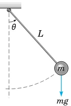
A simple physical problem that leads to a nonlinear differential equation is the oscillating pendulum. The angleθthat an oscillating pendulum of lengthLmakes with the vertical direction (see Figure 1.3.1) satisfies the equation
d2θ
dt2 + g
L sinθ =0, (12)
whose derivation is outlined in Problem 29. The presence of the term involving sinθ makes Eq. (12) nonlinear.
The mathematical theory and methods for solving linear equations are highly devel-oped. In contrast, for nonlinear equations the theory is more complicated and methods of solution are less satisfactory. In view of this, it is fortunate that many significant problems lead to linear ordinary differential equations or can be approximated by linear equations. For example, for the pendulum, if the angleθ is small, then sinθ ∼=θ and Eq. (12) can be approximated by the linear equation
d2θ
dt2 + g
Lθ =0. (13)
This process of approximating a nonlinear equation by a linear one is called lineariza-tionand it is an extremely valuable way to deal with nonlinear equations. Neverthe-less, there are many physical phenomena that simply cannot be represented adequately
L
m
mg
θ