A First course in Differential Equations

NINTH EDITION

A FIRST COURSE IN

DIFFERENTIAL

EQUATIONS

NINTH EDITION

A FIRST COURSE IN

DIFFERENTIAL

EQUATIONS

with Modeling Applications

DENNIS G. ZILL

Loyola Marymount University

Printed in Canada

1 2 3 4 5 6 7 12 11 10 09 08 A First Course in Differential Equations with Modeling Applications, Ninth Edition Dennis G. Zill

Executive Editor: Charlie Van Wagner Development Editor: Leslie Lahr Assistant Editor: Stacy Green Editorial Assistant: Cynthia Ashton Technology Project Manager: Sam

Subity

Marketing Specialist: Ashley Pickering Marketing Communications Manager:

Darlene Amidon-Brent Project Manager, Editorial

Production: Cheryll Linthicum Creative Director: Rob Hugel Art Director: Vernon Boes Print Buyer: Rebecca Cross Permissions Editor: Mardell Glinski

Schultz

Production Service: Hearthside Publishing Services Text Designer: Diane Beasley Photo Researcher: Don Schlotman Copy Editor: Barbara Willette Illustrator: Jade Myers, Matrix Cover Designer: Larry Didona

Cover Image: © Adastra/Getty Images Compositor: ICC Macmillan Inc.

© 2009, 2005 Brooks/Cole, Cengage Learning

ALL RIGHTS RESERVED. No part of this work covered by the copyright herein may be reproduced, transmitted, stored, or used in any form or by any means graphic, electronic, or mechanical, including but not limited to photocopying, recording, scanning, digitizing, taping, Web distribution, information networks, or information storage and retrieval systems, except as permitted under Section 107 or 108 of the 1976 United States Copyright Act, without the prior written permission of the publisher.

Library of Congress Control Number: 2008924906

ISBN-13: 978-0-495-10824-5 ISBN-10: 0-495-10824-3

Brooks/Cole 10 Davis Drive

Belmont, CA 94002-3098 USA

Cengage Learning is a leading provider of customized learning solutions with office locations around the globe, including Singapore, the United Kingdom, Australia, Mexico, Brazil, and Japan. Locate your local office at international.cengage.com/region.

Cengage Learning products are represented in Canada by Nelson Education, Ltd.

For your course and learning solutions, visit academic.cengage.com.

Purchase any of our products at your local college store or at our preferred online store www.ichapters.com.

For product information and technology assistance, contact us at Cengage Learning Customer & Sales Support, 1-800-354-9706.

For permission to use material from this text or product, submit all requests online at cengage.com/permissions.

3

v

CONTENTS

1

INTRODUCTION TO DIFFERENTIAL EQUATIONS

1

Preface ix

1.1 Definitions and Terminology 2

1.2 Initial-Value Problems 13

1.3 Differential Equations as Mathematical Models 19

CHAPTER 1 IN REVIEW 32

2

FIRST-ORDER DIFFERENTIAL EQUATIONS

34

2.1 Solution Curves Without a Solution 35

2.1.1 Direction Fields 35

2.1.2 Autonomous First-Order DEs 37

2.2 Separable Variables 44

2.3 Linear Equations 53

2.4 Exact Equations 62

2.5 Solutions by Substitutions 70

2.6 A Numerical Method 75

CHAPTER 2 IN REVIEW 80

MODELING WITH FIRST-ORDER DIFFERENTIAL EQUATIONS

82

3.1 Linear Models 83

3.2 Nonlinear Models 94

3.3 Modeling with Systems of First-Order DEs 105

5

4

vi ● _CONTENTS

HIGHER-ORDER DIFFERENTIAL EQUATIONS

117

4.1 Preliminary Theory—Linear Equations 118

4.1.1 Initial-Value and Boundary-Value Problems 118

4.1.2 Homogeneous Equations 120

4.1.3 Nonhomogeneous Equations 125

4.2 Reduction of Order 130

4.3 Homogeneous Linear Equations with Constant Coefficients 133

4.4 Undetermined Coefficients—Superposition Approach 140

4.5 Undetermined Coefficients—Annihilator Approach 150

4.6 Variation of Parameters 157

4.7 Cauchy-Euler Equation 162

4.8 Solving Systems of Linear DEs by Elimination 169

4.9 Nonlinear Differential Equations 174

CHAPTER 4 IN REVIEW 178

MODELING WITH HIGHER-ORDER DIFFERENTIAL EQUATIONS

181

5.1 Linear Models: Initial-Value Problems 182

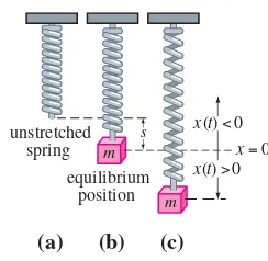
5.1.1 Spring/Mass Systems: Free Undamped Motion 182

5.1.2 Spring/Mass Systems: Free Damped Motion 186

5.1.3 Spring/Mass Systems: Driven Motion 189

5.1.4 Series Circuit Analogue 192

5.2 Linear Models: Boundary-Value Problems 199

5.3 Nonlinear Models 207

CHAPTER 5 IN REVIEW 216

SERIES SOLUTIONS OF LINEAR EQUATIONS

219

6.1 Solutions About Ordinary Points 220

6.1.1 Review of Power Series 220

6.1.2 Power Series Solutions 223

6.2 Solutions About Singular Points 231

6.3 Special Functions 241

6.3.1 Bessel’s Equation 241

6.3.2 Legendre’s Equation 248

CHAPTER 6 IN REVIEW 253

CONTENTS ● vii

7

THE LAPLACE TRANSFORM

255

7.1 Definition of the Laplace Transform 256

7.2 Inverse Transforms and Transforms of Derivatives 262

7.2.1 Inverse Transforms 262

7.2.2 Transforms of Derivatives 265

7.3 Operational Properties I 270

7.3.1 Translation on the s-Axis 271

7.3.2 Translation on the t-Axis 274

7.4 Operational Properties II 282

7.4.1 Derivatives of a Transform 282

7.4.2 Transforms of Integrals 283

7.4.3 Transform of a Periodic Function 287

7.5 The Dirac Delta Function 292

7.6 Systems of Linear Differential Equations 295

CHAPTER 7 IN REVIEW 300

8

SYSTEMS OF LINEAR FIRST-ORDER DIFFERENTIAL EQUATIONS

303

8.1 Preliminary Theory—Linear Systems 304

8.2 Homogeneous Linear Systems 311

8.2.1 Distinct Real Eigenvalues 312

8.2.2 Repeated Eigenvalues 315

8.2.3 Complex Eigenvalues 320

8.3 Nonhomogeneous Linear Systems 326

8.3.1 Undetermined Coefficients 326

8.3.2 Variation of Parameters 329

8.4 Matrix Exponential 334

CHAPTER 8 IN REVIEW 337

9

NUMERICAL SOLUTIONS OF ORDINARY DIFFERENTIAL EQUATIONS

339

9.1 Euler Methods and Error Analysis 340

9.2 Runge-Kutta Methods 345

9.3 Multistep Methods 350

9.4 Higher-Order Equations and Systems 353

9.5 Second-Order Boundary-Value Problems 358

viii ● _CONTENTS

APPENDICES

I Gamma Function APP-1

II Matrices APP-3

III Laplace Transforms APP-21

Answers for Selected Odd-Numbered Problems ANS-1

ix

TO THE STUDENT

Authors of books live with the hope that someone actually readsthem. Contrary to what you might believe, almost everything in a typical college-level mathematics text is written for you and not the instructor. True, the topics covered in the text are cho-sen to appeal to instructors because they make the decision on whether to use it in their classes, but everything written in it is aimed directly at you the student. So I want to encourage you—no, actually I want to tellyou—to read this textbook! But do not read this text like you would a novel; you should not read it fast and you should not skip anything. Think of it as a workbook. By this I mean that mathemat-ics should always be read with pencil and paper at the ready because, most likely, you will have to workyour way through the examples and the discussion. Read—oops, work—all the examples in a section before attempting any of the exercises; the ex-amples are constructed to illustrate what I consider the most important aspects of the section, and therefore, reflect the procedures necessary to work most of the problems in the exercise sets. I tell my students when reading an example, cover up the solu-tion; try working it first, compare your work against the solution given, and then resolve any differences. I have tried to include most of the important steps in each example, but if something is not clear you should always try—and here is where the pencil and paper come in again—to fill in the details or missing steps. This may not be easy, but that is part of the learning process. The accumulation of facts fol-lowed by the slow assimilation of understanding simply cannot be achieved without a struggle.

Specifically for you, a Student Resource and Solutions Manual(SRSM) is avail-able as an optional supplement. In addition to containing solutions of selected prob-lems from the exercises sets, the SRSMhas hints for solving problems, extra exam-ples, and a review of those areas of algebra and calculus that I feel are particularly important to the successful study of differential equations. Bear in mind you do not have to purchase the SRSM; by following my pointers given at the beginning of most sections, you can review the appropriate mathematics from your old precalculus or calculus texts.

In conclusion, I wish you good luck and success. I hope you enjoy the text and the course you are about to embark on—as an undergraduate math major it was one of my favorites because I liked mathematics that connected with the physical world. If you have any comments, or if you find any errors as you read/work your way through the text, or if you come up with a good idea for improving either it or the

SRSM, please feel free to either contact me or my editor at Brooks/Cole Publishing Company:

charlie.vanwagner@cengage.com

TO THE INSTRUCTOR

WHAT IS NEW IN THIS EDITION?

First, let me say what has notchanged. The chapter lineup by topics, the number and order of sections within a chapter, and the basic underlying philosophy remain the same as in the previous editions.

In case you are examining this text for the first time, A First Course in Differential Equations with Modeling Applications, 9th Edition, is intended for either a one-semester or a one-quarter course in ordinary differential equations. The longer version of the text, Differential Equations with Boundary-Value Problems, 7th Edition, can be used for either a one-semester course, or a two-semester course covering ordinary and partial differential equations. This longer text includes six more chapters that cover plane autonomous systems and stability, Fourier series and Fourier transforms, linear partial differential equations and boundary-value prob-lems, and numerical methods for partial differential equations. For a one semester course, I assume that the students have successfully completed at least two semes-ters of calculus. Since you are reading this, undoubtedly you have already examined the table of contents for the topics that are covered. You will not find a “suggested syllabus” in this preface; I will not pretend to be so wise as to tell other teachers what to teach. I feel that there is plenty of material here to pick from and to form a course to your liking. The text strikes a reasonable balance between the analytical, qualitative, and quantitative approaches to the study of differential equations. As far as my “underlying philosophy” it is this: An undergraduate text should be written with the student’s understanding kept firmly in mind, which means to me that the material should be presented in a straightforward, readable, and helpful manner, while keeping the level of theory consistent with the notion of a “first course.”

For those who are familiar with the previous editions, I would like to mention a few of the improvements made in this edition.

• Contributed Problems Selected exercise sets conclude with one or two con-tributed problems. These problems were class-tested and submitted by in-structors of differential equations courses and reflect how they supplement their classroom presentations with additional projects.

• ExercisesMany exercise sets have been updated by the addition of new prob-lems to better test and challenge the students. In like manner, some exercise sets have been improved by sending some problems into early retirement. • DesignThis edition has been upgraded to a four-color design, which adds

depth of meaning to all of the graphics and emphasis to highlighted phrases. I oversaw the creation of each piece of art to ensure that it is as mathemati-cally correct as the text.

• New Figure NumerationIt took many editions to do so, but I finally became convinced that the old numeration of figures, theorems, and definitions had to be changed. In this revision I have utilized a double-decimal numeration sys-tem. By way of illustration, in the last edition Figure 7.52 only indicates that it is the 52nd figure in Chapter 7. In this edition, the same figure is renumbered as Figure 7.6.5, where

ChapterSection

7.6.5 Fifth figure in the section

I feel that this system provides a clearer indication to where things are, with-out the necessity of adding a cumbersome page number.

• Projects from Previous Editions Selected projects and essays from past editions of the textbook can now be found on the companion website at academic.cengage.com/math/zill.

STUDENT RESOURCES

• Student Resource and Solutions Manual, by Warren S. Wright, Dennis G. Zill, and Carol D. Wright (ISBN 0495385662 (accompanies A First Course in Differential Equations with Modeling Applications, 9e), 0495383163 (ac-companies Differential Equations with Boundary-Value Problems, 7e)) pro-vides reviews of important material from algebra and calculus, the solution of every third problem in each exercise set (with the exception of the Discussion

PREFACE ● xi

Problems and Computer Lab Assignments), relevant command syntax for the computer algebra systems Mathematica and Maple, lists of important con-cepts, as well as helpful hints on how to start certain problems.

• DE Toolsis a suite of simulations that provide an interactive, visual explo-ration of the concepts presented in this text. Visit academic.cengage.com/ math/zill to find out more or contact your local sales representative to ask about options for bundling DE Tools with this textbook.

INSTRUCTOR RESOURCES

• Complete Solutions Manual, by Warren S. Wright and Carol D. Wright (ISBN 049538609X), provides worked-out solutions to all problems in the text. • Test Bank, by Gilbert Lewis (ISBN 0495386065) Contains multiple-choice

and short-answer test items that key directly to the text.

ACKNOWLEDGMENTS

Compiling a mathematics textbook such as this and making sure that its thousands of symbols and hundreds of equations are (mostly) accurate is an enormous task, but since I am called “the author” that is my job and responsibility. But many people besides myself have expended enormous amounts of time and energy in working towards its eventual publication. So I would like to take this opportunity to express my sincerest appreciation to everyone—most of them unknown to me—at Brooks/Cole Publishing Company, at Cengage Learning, and at Hearthside Publication Services who were involved in the publication of this new edition. I would, however, like to sin-gle out a few individuals for special recognition: At Brooks/Cole/Cengage, Cheryll Linthicum, Production Project Manager, for her willingness to listen to an author’s ideas and patiently answering the author’s many questions; Larry Didona for the excellent cover designs; Diane Beasley for the interior design; Vernon Boes for super-vising all the art and design; Charlie Van Wagner, sponsoring editor; Stacy Green for coordinating all the supplements; Leslie Lahr, developmental editor, for her sugges-tions, support, and for obtaining and organizing the contributed problems; and at Hearthside Production Services, Anne Seitz, production editor, who once again put all the pieces of the puzzle together. Special thanks go to John Samons for the outstand-ing job he did reviewoutstand-ing the text and answer manuscript for accuracy.

I also extend my heartfelt appreciation to those individuals who took the time out of their busy academic schedules to submit a contributed problem:

Ben Fitzpatrick, Loyola Marymount University

Layachi Hadji, University of Alabama

Michael Prophet, University of Northern Iowa

Doug Shaw, University of Northern Iowa

Warren S. Wright, Loyola Marymount University

David Zeigler, California State University—Sacramento

Finally, over the years these texts have been improved in a countless number of ways through the suggestions and criticisms of the reviewers. Thus it is fitting to con-clude with an acknowledgement of my debt to the following people for sharing their expertise and experience.

REVIEWERS OF PAST EDITIONS

William Atherton, Cleveland State University

Philip Bacon, University of Florida

Bruce Bayly, University of Arizona

William H. Beyer, University of Akron

Dean R. Brown, Youngstown State University

David Buchthal, University of Akron

Nguyen P. Cac, University of Iowa

T. Chow, California State University—Sacramento

Dominic P. Clemence, North Carolina Agricultural and Technical State University

Pasquale Condo, University of Massachusetts—Lowell

Vincent Connolly, Worcester Polytechnic Institute

Philip S. Crooke, Vanderbilt University

Bruce E. Davis, St. Louis Community College at Florissant Valley

Paul W. Davis, Worcester Polytechnic Institute

Richard A. DiDio, La Salle University

James Draper, University of Florida

James M. Edmondson, Santa Barbara City College

John H. Ellison, Grove City College

Raymond Fabec, Louisiana State University

Donna Farrior, University of Tulsa

Robert E. Fennell, Clemson University

W.E. Fitzgibbon, University of Houston

Harvey J. Fletcher, Brigham Young University

Paul J. Gormley, Villanova

Terry Herdman, Virginia Polytechnic Institute and State University

Zdzislaw Jackiewicz, Arizona State University

S.K. Jain, Ohio University

Anthony J. John, Southeastern Massachusetts University

David C. Johnson, University of Kentucky—Lexington

Harry L. Johnson, V.P.I & S.U.

Kenneth R. Johnson, North Dakota State University

Joseph Kazimir, East Los Angeles College

J. Keener, University of Arizona

Steve B. Khlief, Tennessee Technological University (retired)

C.J. Knickerbocker, St. Lawrence University

Carlon A. Krantz, Kean College of New Jersey

Thomas G. Kudzma, University of Lowell

G.E. Latta, University of Virginia

Cecelia Laurie, University of Alabama

James R. McKinney, California Polytechnic State University

James L. Meek, University of Arkansas

Gary H. Meisters, University of Nebraska—Lincoln

Stephen J. Merrill, Marquette University

Vivien Miller, Mississippi State University

Gerald Mueller, Columbus State Community College

Philip S. Mulry, Colgate University

C.J. Neugebauer, Purdue University

Tyre A. Newton, Washington State University

Brian M. O’Connor, Tennessee Technological University

J.K. Oddson, University of California—Riverside

Carol S. O’Dell, Ohio Northern University

A. Peressini, University of Illinois, Urbana—Champaign

J. Perryman, University of Texas at Arlington

Joseph H. Phillips, Sacramento City College

Jacek Polewczak, California State University Northridge

Nancy J. Poxon, California State University—Sacramento

Robert Pruitt, San Jose State University

K. Rager, Metropolitan State College

F.B. Reis, Northeastern University

Tom Roe, South Dakota State University

Kimmo I. Rosenthal, Union College

Barbara Shabell, California Polytechnic State University

Seenith Sivasundaram, Embry–Riddle Aeronautical University

Don E. Soash, Hillsborough Community College

F.W. Stallard, Georgia Institute of Technology

Gregory Stein, The Cooper Union

M.B. Tamburro, Georgia Institute of Technology

Patrick Ward, Illinois Central College

Warren S. Wright, Loyola Marymount University

Jianping Zhu, University of Akron

Jan Zijlstra, Middle Tennessee State University

Jay Zimmerman, Towson University

REVIEWERS OF THE CURRENT EDITIONS

Layachi Hadji, University of Alabama

Ruben Hayrapetyan, Kettering University

Alexandra Kurepa, North Carolina A&T State University

Dennis G. Zill Los Angeles

NINTH EDITION

A FIRST COURSE IN

DIFFERENTIAL

EQUATIONS

1

1

INTRODUCTION TO DIFFERENTIAL

EQUATIONS

1.1 Definitions and Terminology 1.2 Initial-Value Problems

1.3 Differential Equations as Mathematical Models

CHAPTER 1 IN REVIEW

The words differentialandequationscertainly suggest solving some kind of equation that contains derivatives y,y, . . . . Analogous to a course in algebra and trigonometry, in which a good amount of time is spent solving equations such as

x25x40 for the unknown number x, in this course oneof our tasks will be to solve differential equations such as y 2y y0 for an unknown function

y␾(x).

The preceding paragraph tells something, but not the complete story, about the course you are about to begin. As the course unfolds, you will see that there is more to the study of differential equations than just mastering methods that someone has devised to solve them.

DEFINITIONS AND TERMINOLOGY

REVIEW MATERIAL

● Definition of the derivative

● Rules of differentiation

● Derivative as a rate of change

● First derivative and increasing/decreasing

● Second derivative and concavity

INTRODUCTION The derivative dy兾dxof a function y␾(x) is itself another function ␾(x) found by an appropriate rule. The function is differentiable on the interval (,), and by the Chain Rule its derivative is . If we replace on the right-hand side of the last equation by the symbol y, the derivative becomes

. (1)

Now imagine that a friend of yours simply hands you equation (1) —you have no idea how it was constructed —and asks, What is the function represented by the symbol y? You are now face to face with one of the basic problems in this course:

How do you solve such an equation for the unknown function y␾(x)?

dy

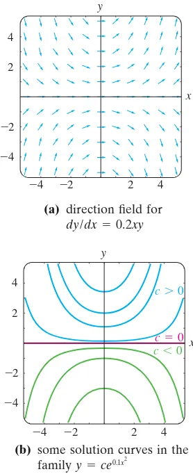
dx0.2xy

e0.1x2 dy>dx0.2xe0.1x2

ye0.1x2 2 ● _{CHAPTER 1 INTRODUCTION TO DIFFERENTIAL EQUATIONS}

1.1

A DEFINITION The equation that we made up in (1) is called a differential equation.Before proceeding any further, let us consider a more precise definition of this concept.

DEFINITION 1.1.1 Differential Equation

An equation containing the derivatives of one or more dependent variables, with respect to one or more independent variables, is said to be a differential equation (DE).

To talk about them, we shall classify differential equations by type, order,and

linearity.

CLASSIFICATION BY TYPE If an equation contains only ordinary derivatives of one or more dependent variables with respect to a single independent variable it is said to be an ordinary differential equation (ODE).For example,

A DE can contain more than one dependent variable

(2)

are ordinary differential equations. An equation involving partial derivatives of one or more dependent variables of two or more independent variables is called a

dy

dx5ye

x_, d

2_y

dx2 dy

dx6y0, and dx

dt

dy

dt 2xy

partial differential equation (PDE).For example,

(3)

are partial differential equations.*

Throughout this text ordinary derivatives will be written by using either the

Leibniz notationdy兾dx,d2y兾dx2,d3y兾dx3, . . . or theprime notationy,y,y, . . . . By using the latter notation, the first two differential equations in (2) can be written a little more compactly as y 5yex_{and y y 6y0. Actually, the prime} notation is used to denote only the first three derivatives; the fourth derivative is writteny(4)instead of y. In general, the nth derivative of yis written dn_y兾dxn_ory(n)_. Although less convenient to write and to typeset, the Leibniz notation has an advan-tage over the prime notation in that it clearly displays both the dependent and independent variables. For example, in the equation

it is immediately seen that the symbol x now represents a dependent variable, whereas the independent variable is t. You should also be aware that in physical sciences and engineering, Newton’s dot notation(derogatively referred to by some as the “flyspeck” notation) is sometimes used to denote derivatives with respect to time t. Thus the differential equation d2s兾dt2 32 becomes ¨s 32. Partial derivatives are often denoted by a subscript notation indicating the indepen-dent variables. For example, with the subscript notation the second equation in (3) becomes uxxutt2ut.

CLASSIFICATION BY ORDER The order of a differential equation (either ODE or PDE) is the order of the highest derivative in the equation. For example,

is a second-order ordinary differential equation. First-order ordinary differential equations are occasionally written in differential form M(x,y)dxN(x,y)dy0.

For example, if we assume that y denotes the dependent variable in

(yx)dx4x dy0, then y dy兾dx, so by dividing by the differential dx, we get the alternative form 4xy yx. See the Remarksat the end of this section.

In symbols we can express an nth-order ordinary differential equation in one dependent variable by the general form

, (4)

whereFis a real-valued function of n2 variables: x,y,y, . . . , y(n)_{. For both} prac-tical and theoreprac-tical reasons we shall also make the assumption hereafter that it is possible to solve an ordinary differential equation in the form (4) uniquely for the

F(x, y, y, . . . , y(n)₎₀

first order second order

5

( )

_–––dy 3 4y ex

dx d2_y

––––

dx2

d2_x

–––

dt2 16x 0

unknown function or dependent variable

independent variable 2_u

x2 2_u

y20, 2_u

x2 2_u

t2 2 u

t, and u y

v x

1.1 DEFINITIONS AND TERMINOLOGY ● 3

*_{Except for this introductory section, only ordinary differential equations are considered in A First}

Course in Differential Equations with Modeling Applications,Ninth Edition. In that text the wordequationand the abbreviation DE refer only to ODEs. Partial differential equations or PDEs are considered in the expanded volume Differential Equations with Boundary-Value Problems,

highest derivative y(n) _{in terms of the remaining n1 variables. The differential} equation

, (5)

wherefis a real-valued continuous function, is referred to as the normal form of (4). Thus when it suits our purposes, we shall use the normal forms

to represent general first- and second-order ordinary differential equations. For example, the normal form of the first-order equation 4xy yxisy (xy)兾4x; the normal form of the second-order equation y y 6y0 is y y 6y. See the Remarks.

CLASSIFICATION BY LINEARITY Annth-order ordinary differential equation (4) is said to be linearifFis linear in y,y, . . . ,y(n). This means that an nth-order ODE is linear when (4) is an(x)y(n)an1(x)y(n1) a1(x)y a0(x)yg(x)0 or

. (6)

Two important special cases of (6) are linear first-order (n1) and linear second-order (n2) DEs:

. (7)

In the additive combination on the left-hand side of equation (6) we see that the char-acteristic two properties of a linear ODE are as follows:

• The dependent variable yand all its derivatives y,y, . . . , y(n)_{are of the} first degree, that is, the power of each term involving yis 1.

• The coefficients a0,a1, . . . , anofy,y, . . . , y(n)depend at most on the independent variable x.

The equations

are, in turn, linear first-, second-, and third-order ordinary differential equations. We have just demonstrated that the first equation is linear in the variable yby writing it in the alternative form 4xy yx. A nonlinearordinary differential equation is sim-ply one that is not linear. Nonlinear functions of the dependent variable or its deriva-tives, such as sin yor , cannot appear in a linear equation. Therefore

are examples of nonlinear first-, second-, and fourth-order ordinary differential equa-tions, respectively.

SOLUTIONS As was stated before, one of the goals in this course is to solve, or find solutions of, differential equations. In the next definition we consider the con-cept of a solution of an ordinary differential equation.

nonlinear term: coefficient depends on y

nonlinear term: nonlinear function of y

nonlinear term: power not 1

(1y)y 2yex_, d _{siny 0, and}

2_y

––––

dx2 y2 0

d4_y

––––

dx4

ey

(yx)dx4x dy0, y 2y y0, and d3y dx3x

dy

dx5ye

x

a₁(x)dy

dxa0(x)yg(x) and a2(x) d2y dx2a1(x)

dy

dxa0(x)yg(x) a_n(x)d

n_y

dxnan1(x)

dn1_y

dxn1 a1(x)

dy

dxa0(x)yg(x) dy

dxf(x,y) and d2_y

dx2f(x,y,y) dn_y

dxnf(x,y,y, . . . , y

(n1)₎

DEFINITION 1.1.2 Solution of an ODE

Any function ␾, defined on an interval Iand possessing at least nderivatives that are continuous on I, which when substituted into an nth-order ordinary differential equation reduces the equation to an identity, is said to be a

solutionof the equation on the interval.

In other words, a solution of an nth-order ordinary differential equation (4) is a func-tion␾that possesses at least nderivatives and for which

We say that ␾satisfiesthe differential equation on I.For our purposes we shall also assume that a solution ␾is a real-valued function. In our introductory discussion we saw that is a solution of dy兾dx0.2xyon the interval (,).

Occasionally, it will be convenient to denote a solution by the alternative symboly(x).

INTERVAL OF DEFINITION You cannot think solutionof an ordinary differential equation without simultaneously thinking interval.The interval Iin Definition 1.1.2 is variously called the interval of definition,theinterval of existence,theinterval of validity,or the domain of the solutionand can be an open interval (a,b), a closed interval [a,b], an infinite interval (a,), and so on.

EXAMPLE 1

Verification of a Solution

Verify that the indicated function is a solution of the given differential equation on the interval (,).

(a) (b)

SOLUTION One way of verifying that the given function is a solution is to see, after substituting, whether each side of the equation is the same for every xin the interval.

(a) From

we see that each side of the equation is the same for every real number x.Note that is, by definition, the nonnegative square root of .

(b) From the derivatives y xex_ex_{andy xe}x_2ex_{we have, for every real} numberx,

Note, too, that in Example 1 each differential equation possesses the constant so-lutiony0, x . A solution of a differential equation that is identically zero on an interval Iis said to be a trivial solution.

SOLUTION CURVE The graph of a solution ␾ of an ODE is called a solution curve.Since␾is a differentiable function, it is continuous on its interval Iof defini-tion. Thus there may be a difference between the graph of the function␾and the

right-hand side:

0.

left-hand side:

y 2y y(xex_2ex_)2(xex_ex_)xex_0,

1 16 x4

y1/21₄x2

right-hand side: xy1/2xⴢ

冢

1

16x

4

冣

1/2_xⴢ

冢

1

4x

2

冣

1

4x

3_,

left-hand side: dy

dx

1 16 (4ⴢx

3₎1

4x

3_,

y 2y y0; yxex

dy>dxxy1/2; y₁₆ 1x4 ye0.1x2

F(x,(x),(x), . . . , (n)_{(x))0 for all x in I.}

graph of the solution␾. Put another way, the domain of the function ␾need not be the same as the interval I of definition (or domain) of the solution ␾. Example 2 illustrates the difference.

EXAMPLE 2

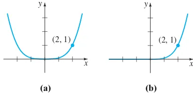
Function versus Solution

The domain of y1兾x, considered simply as a function, is the set of all real num-bers xexcept 0. When we graph y1兾x, we plot points in the xy-plane corre-sponding to a judicious sampling of numbers taken from its domain. The rational functiony1兾xis discontinuous at 0, and its graph, in a neighborhood of the ori-gin, is given in Figure 1.1.1(a). The function y1兾xis not differentiable at x0, since the y-axis (whose equation is x0) is a vertical asymptote of the graph.

Now y1兾x is also a solution of the linear first-order differential equation

xy y0. (Verify.) But when we say that y1兾xis a solutionof this DE, we mean that it is a function defined on an interval Ion which it is differentiable and satisfies the equation. In other words, y1兾xis a solution of the DE on any inter-val that does not contain 0, such as (3,1), , (, 0), or (0, ). Because

the solution curves defined by y1兾xfor3x 1 and are

sim-ply segments, or pieces, of the solution curves defined by y1兾xfor x0 and 0x , respectively, it makes sense to take the interval Ito be as large as possible. Thus we take Ito be either (, 0) or (0, ). The solution curve on (0,) is shown in Figure 1.1.1(b).

EXPLICIT AND IMPLICIT SOLUTIONS You should be familiar with the terms

explicit functionsandimplicit functionsfrom your study of calculus. A solution in which the dependent variable is expressed solely in terms of the independent variable and constants is said to be an explicit solution.For our purposes, let us think of an explicit solution as an explicit formula y␾(x) that we can manipulate, evaluate, and differentiate using the standard rules. We have just seen in the last two examples that , yxex, and y1兾x are, in turn, explicit solutions ofdy兾dxxy1/2,y 2y y0, and xy y0. Moreover, the trivial solu-tion y0 is an explicit solution of all three equations. When we get down to the business of actually solving some ordinary differential equations, you will see that methods of solution do not always lead directly to an explicit solution

y ␾(x). This is particularly true when we attempt to solve nonlinear first-order differential equations. Often we have to be content with a relation or expression

G(x,y)0 that defines a solution ␾implicitly.

DEFINITION 1.1.3 Implicit Solution of an ODE

A relation G(x, y)0 is said to be an implicit solution of an ordinary differential equation (4) on an interval I, provided that there exists at least one function ␾that satisfies the relation as well as the differential equation onI.

It is beyond the scope of this course to investigate the conditions under which a relationG(x,y)0 defines a differentiable function ␾. So we shall assume that if the formal implementation of a method of solution leads to a relation G(x,y)0, then there exists at least one function ␾ that satisfies both the relation (that is,

G(x,␾(x))0) and the differential equation on an interval I.If the implicit solution

G(x,y)0 is fairly simple, we may be able to solve for yin terms of xand obtain one or more explicit solutions. See the Remarks.

y₁₆ 1x4

1

2x10

(

1 2, 10

)

6 ● CHAPTER 1 INTRODUCTION TO DIFFERENTIAL EQUATIONS

1

x y

1

(a) functiony1/x,x苷₀

(b) solutiony1/x, (0,앝) 1

x y

1

FIGURE 1.1.1 The function y1兾x

EXAMPLE 3

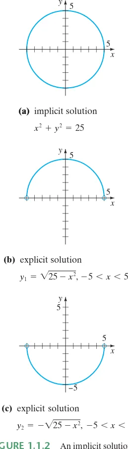
Verification of an Implicit Solution

The relation x2y225 is an implicit solution of the differential equation

(8)

on the open interval (5, 5). By implicit differentiation we obtain

.

Solving the last equation for the symbol dy兾dx gives (8). Moreover, solving

x2y225 for y in terms of x yields . The two functions

and satisfy the relation (that is,

x2␾1225 and x2␾2225) and are explicit solutions defined on the interval (5, 5). The solution curves given in Figures 1.1.2(b) and 1.1.2(c) are segments of the graph of the implicit solution in Figure 1.1.2(a).

Any relation of the form x2y2c0formallysatisfies (8) for any constant c.

However, it is understood that the relation should always make sense in the real number system; thus, for example, if c 25, we cannot say that x2y2250 is an implicit solution of the equation. (Why not?)

Because the distinction between an explicit solution and an implicit solution should be intuitively clear, we will not belabor the issue by always saying, “Here is an explicit (implicit) solution.”

FAMILIES OF SOLUTIONS The study of differential equations is similar to that of integral calculus. In some texts a solution ␾is sometimes referred to as an integral

of the equation, and its graph is called an integral curve.When evaluating an anti-derivative or indefinite integral in calculus, we use a single constant cof integration. Analogously, when solving a first-order differential equation F(x, y, y)0, we

usually obtain a solution containing a single arbitrary constant or parameter c. A solution containing an arbitrary constant represents a set G(x,y,c)0 of solutions called a one-parameter family of solutions.When solving an nth-order differential equation F(x, y, y, . . . ,y(n)_{)0, we seek an n-parameter family of solutions}

G(x,y,c1,c2, . . . , cn)0. This means that a single differential equation can possess an infinite number of solutionscorresponding to the unlimited number of choices for the parameter(s). A solution of a differential equation that is free of arbitrary parameters is called a particular solution.For example, the one-parameter family

y cxxcosxis an explicit solution of the linear first-order equation xy y x2sinxon the interval (,). (Verify.) Figure 1.1.3, obtained by using graphing soft-ware, shows the graphs of some of the solutions in this family. The solution y xcosx, the blue curve in the figure, is a particular solution corresponding to c0. Similarly, on the interval (,),yc1exc2xexis a two-parameter family of solu-tions of the linear second-order equation y 2y y0 in Example 1. (Verify.) Some particular solutions of the equation are the trivial solution y0 (c1c20),

yxex_(c

10,c21),y5ex2xex(c15,c2 2), and so on.

Sometimes a differential equation possesses a solution that is not a member of a family of solutions of the equation —that is, a solution that cannot be obtained by spe-cializinganyof the parameters in the family of solutions. Such an extra solution is called asingular solution.For example, we have seen that and y0 are solutions of the differential equation dy兾dxxy1/2on (,). In Section 2.2 we shall demonstrate, by actually solving it, that the differential equation dy兾dxxy1/2possesses the one-parameter family of solutions . When c0, the resulting particular solution is y₁₆ 1x4. But notice that the trivial solution y0 is a singular solution, since

y

(

1₄x2c

)

2

y₁₆ 1x4 y2(x) 125x2 y1(x) 125x2

y 225x2

d dxx

2 d

dxy

2 d

dx 25 or 2x2y dy

dx0

dy dx

x y

1.1 DEFINITIONS AND TERMINOLOGY ● 7

y

x 5 5

y

x 5 5

y

x 5 5

−5

(a) implicit solution

x2_y2₂₅

(b) explicit solution

y1兹25x2,5x5

(c) explicit solution

y2 兹25x2,5x5

(a)

FIGURE 1.1.2 An implicit solution and two explicit solutions of y x兾y

FIGURE 1.1.3 Some solutions of

xy yx2sinx

y

x c > 0

it is not a member of the family ; there is no way of assigning a value to the constant cto obtain y0.

In all the preceding examples we used xandyto denote the independent and dependent variables, respectively. But you should become accustomed to seeing and working with other symbols to denote these variables. For example, we could denote the independent variable by tand the dependent variable by x.

EXAMPLE 4

Using Different Symbols

The functions xc1cos 4tandxc2sin 4t, where c1andc2are arbitrary constants or parameters, are both solutions of the linear differential equation

For xc1cos 4tthe first two derivatives with respect to tarex 4c1sin 4t andx 16c1cos 4t.Substitutingxandxthen gives

In like manner, for xc2sin 4twe have x 16c2sin 4t, and so

Finally, it is straightforward to verify that the linear combination of solutions, or the two-parameter family xc1cos 4tc2sin 4t, is also a solution of the differential equation.

The next example shows that a solution of a differential equation can be a piecewise-defined function.

EXAMPLE 5

A Piecewise-Defined Solution

You should verify that the one-parameter family ycx4is a one-parameter family of solutions of the differential equation xy 4y0 on the inverval (,). See Figure 1.1.4(a). The piecewise-defined differentiable function

is a particular solution of the equation but cannot be obtained from the family

ycx4by a single choice of c; the solution is constructed from the family by choos-ingc 1 for x0 and c1 for x0. See Figure 1.1.4(b).

SYSTEMS OF DIFFERENTIAL EQUATIONS Up to this point we have been discussing single differential equations containing one unknown function. But often in theory, as well as in many applications, we must deal with systems of differential equations. Asystem of ordinary differential equationsis two or more equations involving the derivatives of two or more unknown functions of a single independent variable. For example, if x and y denote dependent variables and t

denotes the independent variable, then a system of two first-order differential equations is given by

(9)

dy

dt g(t,x,y). dx

dt f(t,x,y) y

冦

x

4_{, x0}

x4, x0

x 16x 16c₂sin 4t16(c₂ sin 4t)0.

x 16x 16c1cos 4t16(c1 cos 4t)0.

x 16x0.

y

(

1₄x2c

)

2 8 ● _{CHAPTER 1 INTRODUCTION TO DIFFERENTIAL EQUATIONS}

FIGURE 1.1.4 Some solutions of

xy 4y0

(a)two explicit solutions

(b)piecewise-defined solution c =1

c = −1 x y

c =1, x ≤ 0

c = −1, x < 0

Asolutionof a system such as (9) is a pair of differentiable functions x␾1(t),

y␾2(t), defined on a common interval I, that satisfy each equation of the system on this interval.

REMARKS

(i) A few last words about implicit solutions of differential equations are in order. In Example 3 we were able to solve the relation x2y225 for

y in terms of x to get two explicit solutions, and

, of the differential equation (8). But don’t read too much into this one example. Unless it is easy or important or you are instructed to, there is usually no need to try to solve an implicit solution G(x,y)0 for y

explicitly in terms of x.Also do not misinterpret the second sentence following Definition 1.1.3. An implicit solution G(x,y)0 can define a perfectly good differentiable function ␾that is a solution of a DE, yet we might not be able to solve G(x,y)0 using analytical methods such as algebra. The solution curve of␾may be a segment or piece of the graph of G(x,y)0. See Problems 45 and 46 in Exercises 1.1. Also, read the discussion following Example 4 in Section 2.2.

(ii) Although the concept of a solution has been emphasized in this section, you should also be aware that a DE does not necessarily have to possess a solution. See Problem 39 in Exercises 1.1. The question of whether a solution exists will be touched on in the next section.

(iii) It might not be apparent whether a first-order ODE written in differential formM(x,y)dxN(x,y)dy0 is linear or nonlinear because there is nothing in this form that tells us which symbol denotes the dependent variable. See Problems 9 and 10 in Exercises 1.1.

(iv) It might not seem like a big deal to assume that F(x,y,y, . . . , y(n)_{)0 can} be solved for y(n), but one should be a little bit careful here. There are exceptions, and there certainly are some problems connected with this assumption. See Problems 52 and 53 in Exercises 1.1.

(v) You may run across the term closed form solutions in DE texts or in lectures in courses in differential equations. Translated, this phrase usually refers to explicit solutions that are expressible in terms of elementary (or familiar) functions:finite combinations of integer powers of x, roots, exponen-tial and logarithmic functions, and trigonometric and inverse trigonometric functions.

(vi) If everysolution of an nth-order ODE F(x,y,y, . . . , y(n))0 on an inter-val Ican be obtained from an n-parameter family G(x,y,c1,c2, . . . ,cn)0 by appropriate choices of the parameters ci,i1, 2, . . . , n, we then say that the family is the general solutionof the DE. In solving linear ODEs, we shall im-pose relatively simple restrictions on the coefficients of the equation; with these restrictions one can be assured that not only does a solution exist on an interval but also that a family of solutions yields all possible solutions. Nonlinear ODEs, with the exception of some first-order equations, are usually difficult or impos-sible to solve in terms of elementary functions. Furthermore, if we happen to obtain a family of solutions for a nonlinear equation, it is not obvious whether this family contains all solutions. On a practical level, then, the designation “general solution” is applied only to linear ODEs. Don’t be concerned about this concept at this point, but store the words “general solution” in the back of your mind —we will come back to this notion in Section 2.3 and again in Chapter 4.

2(x) 125x2

10 ● CHAPTER 1 INTRODUCTION TO DIFFERENTIAL EQUATIONS

EXERCISES 1.1

Answers to selected odd-numbered problems begin on page ANS-1.

In Problems 1 – 8 state the order of the given ordinary differ-ential equation. Determine whether the equation is linear or nonlinear by matching it with (6).

1. (1x)y 4xy5ycosx

2.

3. t5y(4)t3y 6y0

4.

5.

6.

7. (sin␪)y (cos␪)y 2

8.

In Problems 9 and 10 determine whether the given first-order differential equation is linear in the indicated dependent variable by matching it with the first differential equation given in (7).

9. (y21)dxx dy0; in y; in x

10. u dv(vuvueu_{)du0; in v; in u}

In Problems 11 –14 verify that the indicated function is an explicit solution of the given differential equation. Assume an appropriate interval Iof definition for each solution.

11. 2y y0; yex/2

12.

13. y 6y 13y0; ye3xcos 2x

14. y ytanx; y (cosx)ln(secxtanx)

In Problems 15 – 18 verify that the indicated function

y␾(x) is an explicit solution of the given first-order differential equation. Proceed as in Example 2, by consider-ing␾simply as afunction,give its domain. Then by consid-ering␾as a solutionof the differential equation, give at least one interval Iof definition.

15. (yx)y yx8; yx42x2

dy

dt 20y24; y

6 5 6 5e 20t ¨

x

冢

1x

.2

3

冣

x .

x0

d2R dt2

k R2 d2y

dx2 B1

冢

dy dx

冣

2

d2u dr2

du

drucos(ru) xd

3_y

dx3

冢

dy dx

冣

4

y0

16. y 25y2; y5 tan 5x

17. y 2xy2; y1兾(4x2)

18. 2y y3cosx; y(1sinx)1/2

In Problems 19 and 20 verify that the indicated expression is an implicit solution of the given first-order differential equa-tion. Find at least one explicit solution y␾(x) in each case. Use a graphing utility to obtain the graph of an explicit solu-tion. Give an interval Iof definition of each solution ␾.

19.

20. 2xy dx(x2y)dy0; 2x2yy21

In Problems 21 –24 verify that the indicated family of func-tions is a solution of the given differential equation. Assume an appropriate interval Iof definition for each solution.

21.

22.

23.

24.

25. Verify that the piecewise-defined function

is a solution of the differential equation xy 2y0 on (,).

26. In Example 3 we saw that y␾1(x) and

are solutions of dy兾dx x兾yon the interval (5, 5). Explain why the piecewise-defined function

is not a solution of the differential equation on the interval (5, 5).

y

冦

125x

2_,

125x2,

5x0

0x5

y2(x) 125x2

125x2 y

冦

x

2_{, x0}

x2_{, x0}

yc1x1c2xc3x ln x4x2

x3d

3_y

dx32x

2d2y

dx2x dy

dxy12x

2_;

d2_y

dx24 dy

dx4y0; yc1e

2x_c

2xe2x

dy

dx2xy1; ye

x2

冕

x

0

et2

dtc₁ex2 dP

dt P(1P); P c₁et

1c₁et

dX

dt (X1)(12X); ln

冢

2X1

In Problems 27–30 find values of m so that the function

yemxis a solution of the given differential equation.

27. y 2y0 28. 5y 2y

29. y 5y 6y0 30. 2y 7y 4y0

In Problems 31 and 32 find values of mso that the function

yxm_{is a solution of the given differential equation.}

31. xy 2y 0

32. x2y 7xy 15y0

In Problems 33– 36 use the concept that yc, x , is a constant function if and only if y 0 to determine whether the given differential equation possesses constant solutions.

33. 3xy 5y10

34. y y22y3

35. (y1)y 1

36. y 4y 6y10

In Problems 37 and 38 verify that the indicated pair of functions is a solution of the given system of differential equations on the interval (,).

37. 38.

,

Discussion Problems

39. Make up a differential equation that does not possess any real solutions.

40. Make up a differential equation that you feel confident possesses only the trivial solution y0. Explain your reasoning.

41. What function do you know from calculus is such that its first derivative is itself? Its first derivative is a constant multiple k of itself? Write each answer in the form of a first-order differential equation with a solution.

42. What function (or functions) do you know from calcu-lus is such that its second derivative is itself? Its second derivative is the negative of itself? Write each answer in the form of a second-order differential equation with a solution.

y cos 2tsin 2t1₅et

y e2t_5e6t

xcos 2tsin 2t1₅et

xe2t_3e6t_,

d2y

dt24xe

t_;

dy

dt 5x3y;

d2x

dt24ye

t

dx

dt x3y

1.1 DEFINITIONS AND TERMINOLOGY ● 11

43. Given that ysin x is an explicit solution of the

first-order differential equation . Find

an interval Iof definition. [Hint: Iisnotthe interval (,).]

44. Discuss why it makes intuitive sense to presume that the linear differential equation y 2y 4y5 sin t

has a solution of the form yAsintBcost, where

A andB are constants. Then find specific constants A

andBso that yAsintBcostis a particular solu-tion of the DE.

In Problems 45 and 46 the given figure represents the graph of an implicit solution G(x,y)0 of a differential equation

dy兾dxf(x, y). In each case the relation G(x, y)0 implicitly defines several solutions of the DE. Carefully reproduce each figure on a piece of paper. Use different colored pencils to mark off segments, or pieces, on each graph that correspond to graphs of solutions. Keep in mind that a solution ␾must be a function and differentiable. Use the solution curve to estimate an interval Iof definition of each solution ␾.

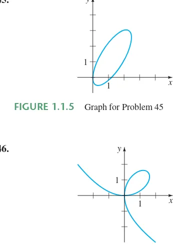
45.

dy

dx 11y

2

FIGURE 1.1.5 Graph for Problem 45

FIGURE 1.1.6 Graph for Problem 46 y

x 1

1

1 x 1

y 46.

47. The graphs of members of the one-parameter family

x3y33cxy are called folia of Descartes. Verify that this family is an implicit solution of the first-order differential equation

dy

dx

y(y32x3)

48. The graph in Figure 1.1.6 is the member of the family of folia in Problem 47 corresponding to c1. Discuss: How can the DE in Problem 47 help in finding points on the graph of x3y33xywhere the tangent line is vertical? How does knowing where a tangent line is vertical help in determining an interval Iof definition of a solution ␾ of the DE? Carry out your ideas, and compare with your estimates of the intervals in Problem 46.

49. In Example 3 the largest interval I over which the explicit solutions y␾1(x) and y␾2(x) are defined is the open interval (5, 5). Why can’t the interval Iof definition be the closed interval [5, 5]?

50. In Problem 21 a one-parameter family of solutions of the DE P P(1P) is given. Does any solution curve pass through the point (0, 3)? Through the point (0, 1)?

51. Discuss, and illustrate with examples, how to solve differential equations of the forms dy兾dxf(x) and

d2y兾dx2f(x).

52. The differential equation x(y)2_{4y 12x}3_{0 has} the form given in (4). Determine whether the equation can be put into the normal form dy兾dxf(x,y).

53. The normal form (5) of an nth-order differential equa-tion is equivalent to (4) whenever both forms have exactly the same solutions. Make up a first-order differ-ential equation for which F(x,y,y)0 is not equiva-lent to the normal form dy兾dxf(x,y).

54. Find a linear second-order differential equation

F(x, y,y,y)0 for which yc1xc2x2 is a two-parameter family of solutions. Make sure that your equa-tion is free of the arbitrary parameters c1andc2.

Qualitative information about a solution y␾(x) of a differential equation can often be obtained from the equation itself. Before working Problems 55– 58, recall the geometric significance of the derivatives dy兾dx

andd2y兾dx2.

55. Consider the differential equation .

(a) Explain why a solution of the DE must be an increasing function on any interval of the x-axis.

(b) What are What does

this suggest about a solution curve as

(c) Determine an interval over which a solution curve is concave down and an interval over which the curve is concave up.

(d) Sketch the graph of a solution y␾(x) of the dif-ferential equation whose shape is suggested by parts (a) – (c).

x:?

lim

x:dy>dx and limx:dy>dx?

dy>dxex2

12 ● CHAPTER 1 INTRODUCTION TO DIFFERENTIAL EQUATIONS

56. Consider the differential equation dy兾dx5y. (a) Either by inspection or by the method suggested in

Problems 33– 36, find a constant solution of the DE.

(b) Using only the differential equation, find intervals on they-axis on which a nonconstant solution y␾(x) is increasing. Find intervals on the y-axis on which

y␾(x) is decreasing.

57. Consider the differential equation dy兾dxy(aby), whereaandbare positive constants.

(a) Either by inspection or by the method suggested in Problems 33– 36, find two constant solutions of the DE.

(b) Using only the differential equation, find intervals on they-axis on which a nonconstant solution y␾(x) is increasing. Find intervals on which y␾(x) is decreasing.

(c) Using only the differential equation, explain why

ya兾2bis the y-coordinate of a point of inflection of the graph of a nonconstant solution y␾(x).

(d) On the same coordinate axes, sketch the graphs of the two constant solutions found in part (a). These constant solutions partition the xy-plane into three regions. In each region, sketch the graph of a non-constant solution y␾(x) whose shape is sug-gested by the results in parts (b) and (c).

58. Consider the differential equation y y24.

(a) Explain why there exist no constant solutions of the DE.

(b) Describe the graph of a solution y␾(x). For example, can a solution curve have any relative extrema?

(c) Explain why y0 is the y-coordinate of a point of inflection of a solution curve.

(d) Sketch the graph of a solution y␾(x) of the differential equation whose shape is suggested by parts (a) –(c).

Computer Lab Assignments

In Problems 59 and 60 use a CAS to compute all derivatives and to carry out the simplifications needed to verify that the indicated function is a particular solution of the given differ-ential equation.

59. y(4)20y 158y 580y 841y0;

yxe5x_{cos 2x}

60.

y20cos(5 ln x)

x 3

sin(5 ln x)

FIRST- AND SECOND-ORDER IVPS The problem given in (1) is also called an

nth-order initial-value problem.For example,

(2)

and ₍₃₎

arefirst-andsecond-orderinitial-value problems, respectively. These two problems are easy to interpret in geometric terms. For (2) we are seeking a solution y(x) of the differential equation y f(x,y) on an interval Icontainingx0so that its graph passes through the specified point (x0,y0). A solution curve is shown in blue in Figure 1.2.1. For (3) we want to find a solution y(x) of the differential equation y f(x,y,y) on an interval Icontainingx0so that its graph not only passes through (x0,y0) but the slope of the curve at this point is the number y1. A solution curve is shown in blue in Figure 1.2.2. The words initial conditionsderive from physical systems where the independent variable is time tand where y(t0)y0andy(t0)y1represent the posi-tion and velocity, respectively, of an object at some beginning, or initial, time t0.

Solving an nth-order initial-value problem such as (1) frequently entails first finding an n-parameter family of solutions of the given differential equation and then using the ninitial conditions at x0to determine numerical values of the nconstants in the family. The resulting particular solution is defined on some interval Icontaining the initial point x0.

EXAMPLE 1

Two First-Order IVPs

In Problem 41 in Exercises 1.1 you were asked to deduce that ycexis a one-parameter family of solutions of the simple first-order equation y y. All the solutions in this family are defined on the interval (,). If we impose an initial condition, say, y(0)3, then substituting x0,y3 in the family determines the

Subject to:

y(x0)y0,y(x0)y1 Solve:

d

2_y

dx2 f(x,y,y) Subject to:

y(x₀)y₀ Solve:

dy

dxf(x,y)

1.2 INITIAL-VALUE PROBLEMS ● 13

INITIAL-VALUE PROBLEMS

REVIEW MATERIAL

● Normal form of a DE

● Solution of a DE

● Family of solutions

INTRODUCTION We are often interested in problems in which we seek a solution y(x) of a differential equation so that y(x) satisfies prescribed side conditions—that is, conditions imposed on the unknown y(x) or its derivatives. On some interval Icontainingx0the problem

(1)

where y0, y1, . . . ,yn1 are arbitrarily specified real constants, is called an initial-value

problem (IVP).The values of y(x) and its first n1 derivatives at a single point x0,y(x0)y0,

y(x0)y1, . . . , y(n1)(x0)yn1, are called initial conditions.

Subject to:

y(x0)y0,y(x0)y1, . . . , y(n1)(x0)yn1,

Solve:

d

n_y

dxnf冢x,y,y, . . . , y

(n1)_冣

1.2

FIGURE 1.2.1 Solution of first-order IVP

FIGURE 1.2.2 Solution of second-order IVP

x I

solutions of the DE

(x₀,y₀)

y

m = y₁ x I

solutions of the DE

(x₀,y₀)

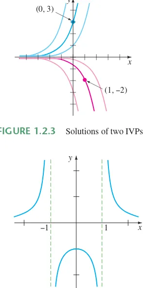
constant 3ce0c.Thusy3ex_{is a solution of the IVP}

Now if we demand that a solution curve pass through the point (1, 2) rather than (0, 3), then y(1) 2 will yield 2ceorc 2e1. In this case y 2ex1_is

a solution of the IVP

The two solution curves are shown in dark blue and dark red in Figure 1.2.3.

The next example illustrates another first-order initial-value problem. In this example notice how the interval Iof definition of the solution y(x) depends on the initial condition y(x0)y0.

EXAMPLE 2

Interval Iof Definition of a Solution

In Problem 6 of Exercises 2.2 you will be asked to show that a one-parameter family of solutions of the first-order differential equation y 2xy20 is y1兾(x2c). If we impose the initial condition y(0) 1, then substituting x0 and y 1 into the family of solutions gives 11�