The most important macroeconomic variable is gross domestic product (GDP). As we have seen, GDP measures both a nation’s total output of goods and ser-vices and its total income.To appreciate the significance of GDP, one need only take a quick look at international data: compared with their poorer counterparts, nations with a high level of GDP per person have everything from better child-hood nutrition to more televisions per household. A large GDP does not ensure that all of a nation’s citizens are happy, but it may be the best recipe for happiness that macroeconomists have to offer.
This chapter addresses four groups of questions about the sources and uses of a nation’s GDP:
➤ How much do the firms in the economy produce? What determines a na-tion’s total income?
➤ Who gets the income from production? How much goes to compensate workers, and how much goes to compensate owners of capital?
➤ Who buys the output of the economy? How much do households pur-chase for consumption, how much do households and firms purpur-chase for investment, and how much does the government buy for public purposes?
➤ What equilibrates the demand for and supply of goods and services? What ensures that desired spending on consumption, investment, and govern-ment purchases equals the level of production?
To answer these questions, we must examine how the various parts of the econ-omy interact.
A good place to start is the circular flow diagram. In Chapter 2 we traced the circular flow of dollars in a hypothetical economy that produced one product, bread, from labor services. Figure 3-1 more accurately reflects how real economies function. It shows the linkages among the economic actors—households, firms,
3
National Income: Where It Comes
From and Where It Goes
C H A P T E R
A large income is the best recipe for happiness I ever heard of.
— Jane Austen
and the government—and how dollars flow among them through the various markets in the economy.
Let’s look at the flow of dollars from the viewpoints of these economic ac-tors. Households receive income and use it to pay taxes to the government, to consume goods and services, and to save through the financial markets. Firms receive revenue from the sale of goods and services and use it to pay for the factors of production. Both households and firms borrow in financial markets to buy investment goods, such as houses and factories. The govern-ment receives revenue from taxes and uses it to pay for governgovern-ment pur-chases. Any excess of tax revenue over government spending is called public saving, which can be either positive (a budget surplus) or negative (a budget deficit).
In this chapter we develop a basic classical model to explain the economic interactions depicted in Figure 3-1. We begin with firms and look at what
f i g u r e 3 - 1
Income
Private saving
Taxes
Consumption Firm revenue
Investment Public
saving
Government purchases
Factor payments Markets for Factors
of Production
Markets for Goods and Services
Financial Markets
Government Firms
Households
determines their level of production (and, thus, the level of national income). Then we examine how the markets for the factors of production distribute this income to households. Next, we consider how much of this income households consume and how much they save. In addition to discussing the demand for goods and services arising from the consumption of households, we discuss the demand arising from investment and government purchases. Finally, we come full circle and examine how the demand for goods and ser-vices (the sum of consumption, investment, and government purchases) and the supply of goods and services (the level of production) are brought into balance.
3-1
What Determines the Total Production of
Goods and Services?
An economy’s output of goods and services—its GDP—depends on (1) its quan-tity of inputs, called the factors of production, and (2) its ability to turn inputs into output, as represented by the production function.We discuss each of these in turn.
The Factors of Production
Factors of productionare the inputs used to produce goods and services.The two most important factors of production are capital and labor. Capital is the set of tools that workers use: the construction worker’s crane, the accountant’s calcu-lator, and this author’s personal computer. Labor is the time people spend work-ing.We use the symbol Kto denote the amount of capital and the symbol Lto denote the amount of labor.
In this chapter we take the economy’s factors of production as given. In other words, we assume that the economy has a fixed amount of capital and a fixed amount of labor.We write
K=K _ . L=L
_ .
The overbar means that each variable is fixed at some level. In Chapter 7 we ex-amine what happens when the factors of production change over time, as they do in the real world. For now, to keep our analysis simple, we assume fixed amounts of capital and labor.
The Production Function
The available production technology determines how much output is produced from given amounts of capital and labor. Economists express the available tech-nology using a production function. Letting Ydenote the amount of output, we write the production function as
Y=F(K,L).
This equation states that output is a function of the amount of capital and the amount of labor.
The production function reflects the available technology for turning capital and labor into output. If someone invents a better way to produce a good, the re-sult is more output from the same amounts of capital and labor.Thus, technolog-ical change alters the production function.
Many production functions have a property called constant returns to scale. A production function has constant returns to scale if an increase of an equal percentage in all factors of production causes an increase in output of the same percentage. If the production function has constant returns to scale, then we get 10 percent more output when we increase both capital and labor by 10 percent. Mathematically, a production function has constant returns to scale if
zY=F(zK,zL)
for any positive number z.This equation says that if we multiply both the amount of capital and the amount of labor by some number z, output is also multiplied by z. In the next section we see that the assumption of constant returns to scale has an important implication for how the income from production is distributed.
As an example of a production function, consider production at a bakery.The kitchen and its equipment are the bakery’s capital, the workers hired to make the bread are its labor, and the loaves of bread are its output.The bakery’s production function shows that the number of loaves produced depends on the amount of equipment and the number of workers. If the production function has constant returns to scale, then doubling the amount of equipment and the number of workers doubles the amount of bread produced.
The Supply of Goods and Services
We can now see that the factors of production and the production function to-gether determine the quantity of goods and services supplied, which in turn equals the economy’s output.To express this mathematically, we write
Y=F(K _
,L _ )
= Y
_ .
discuss economic growth in Chapters 7 and 8, we will examine how increases in capital and labor and improvements in the production technology lead to growth in the economy’s output.
3-2
How Is National Income Distributed to the
Factors of Production?
As we discussed in Chapter 2, the total output of an economy equals its total in-come. Because the factors of production and the production function together determine the total output of goods and services, they also determine national income. The circular flow diagram in Figure 3-1 shows that this national in-come flows from firms to households through the markets for the factors of production.
In this section we continue developing our model of the economy by dis-cussing how these factor markets work. Economists have long studied factor markets to understand the distribution of income. (For example, Karl Marx, the noted nineteenth-century economist, spent much time trying to explain the in-comes of capital and labor. The political philosophy of communism was in part based on Marx’s now-discredited theory.) Here we examine the modern theory of how national income is divided among the factors of production.This theory, called the neoclassical theory of distribution, is accepted by most economists today.
Factor Prices
The distribution of national income is determined by factor prices. Factor prices are the amounts paid to the factors of production—the wage workers earn and the rent the owners of capital collect. As Figure 3-2 illustrates, the price each factor of production receives for its services is in turn determined by the supply and demand for that factor. Because we have assumed that the economy’s factors of production are fixed, the factor supply curve in Figure 3-2 is vertical. The intersection of the downward-sloping factor demand curve and the vertical supply curve determines the equilibrium factor price.
To understand factor prices and the distribution of income, we must examine the demand for the factors of production. Because factor demand arises from the thousands of firms that use capital and labor, we now look at the decisions faced by a typical firm about how much of these factors to employ.
The Decisions Facing the Competitive Firm
much as it wants without causing the price of the good to fall, or it can stop sell-ing altogether without caussell-ing the price of the good to rise. Similarly, our firm cannot influence the wages of the workers it employs because many other local
firms also employ workers.The firm has no reason to pay more than the market wage, and if it tried to pay less, its workers would take jobs elsewhere.Therefore, the competitive firm takes the prices of its output and its inputs as given.
To make its product, the firm needs two factors of production, capital and labor. As we did for the aggregate economy, we represent the firm’s production technology by the production function
Y=F(K,L),
where Y is the number of units produced (the firm’s output),Kthe number of machines used (the amount of capital), and L the number of hours worked by the firm’s employees (the amount of labor).The firm produces more output if it has more machines or if its employees work more hours.
The firm sells its output at a price P, hires workers at a wage W, and rents cap-ital at a rate R. Notice that when we speak of firms renting capital, we are assum-ing that households own the economy’s stock of capital. In this analysis, households rent out their capital, just as they sell their labor. The firm obtains both factors of production from the households that own them.1
The goal of the firm is to maximize profit.Profitis revenue minus costs—it is what the owners of the firm keep after paying for the costs of production. Rev-enue equals P× Y, the selling price of the good P multiplied by the amount of
f i g u r e 3 - 2
Equilibrium factor price
Factor supply
Factor demand
Quantity of factor
Factor price How a Factor of Production Is
Compensated The price paid to any factor of production depends on the supply and de-mand for that factor’s services.
Because we have assumed that supply is fixed, the supply curve
is vertical. The demand curve is downward sloping. The inter-section of supply and demand determines the equilibrium factor price.
1
the good the firm produces Y. Costs include both labor costs and capital costs. Labor costs equal W×L, the wage Wtimes the amount of labor L. Capital costs equal R×K, the rental price of capital Rtimes the amount of capital K.We can write
Profit =Revenue −Labor Costs −Capital Costs
= PY − WL − RK.
To see how profit depends on the factors of production, we use the production function Y=F(K,L) to substitute for Yto obtain
Profit =PF(K,L) −WL−RK.
This equation shows that profit depends on the product price P, the factor prices
W and R, and the factor quantities L and K. The competitive firm takes the product price and the factor prices as given and chooses the amounts of labor and capital that maximize profit.
The Firm’s Demand for Factors
We now know that our firm will hire labor and rent capital in the quantities that maximize profit. But what are those profit-maximizing quantities? To answer this question, we first consider the quantity of labor and then the quantity of capital.
The Marginal Product of Labor The more labor the firm employs, the more output it produces. The marginal product of labor (MPL) is the extra amount of output the firm gets from one extra unit of labor, holding the amount of capital fixed.We can express this using the production function:
MPL=F(K,L+1) −F(K,L).
The first term on the right-hand side is the amount of output produced with K
units of capital and L+1 units of labor; the second term is the amount of output produced with Kunits of capital and Lunits of labor. This equation states that the marginal product of labor is the difference between the amount of output produced with L+1 units of labor and the amount produced with only Lunits of labor.
Most production functions have the property of diminishing marginal product: holding the amount of capital fixed, the marginal product of labor de-creases as the amount of labor inde-creases. Consider again the production of bread at a bakery. As a bakery hires more labor, it produces more bread.The MPLis the amount of extra bread produced when an extra unit of labor is hired. As more labor is added to a fixed amount of capital, however, the MPLfalls. Fewer addi-tional loaves are produced because workers are less productive when the kitchen is more crowded. In other words, holding the size of the kitchen fixed, each ad-ditional worker adds fewer loaves of bread to the bakery’s output.
amount of labor.This figure shows that the marginal product of labor is the slope of the production function. As the amount of labor increases, the production function becomes flatter, indicating diminishing marginal product.
From the Marginal Product of Labor to Labor Demand When the compe-titive, profit-maximizing firm is deciding whether to hire an additional unit of labor, it considers how that decision would affect profits. It therefore compares the extra revenue from the increased production that results from the added labor to the extra cost of higher spending on wages.The increase in revenue from an addi-tional unit of labor depends on two variables: the marginal product of labor and the price of the output. Because an extra unit of labor produces MPL units of output and each unit of output sells for Pdollars, the extra revenue is P×MPL. The extra cost of hiring one more unit of labor is the wage W.Thus, the change in profit from hiring an additional unit of labor is
D
Profit =D
Revenue −D
Cost =(P×MPL) −W.The symbol
D
(called delta) denotes the change in a variable. f i g u r e 3 - 3F(K, L)
Output, Y
Labor, L MPL
1
MPL
1
MPL
1
1. The slope of production function equals marginal product of labor.
2. As more labor is added, the marginal product of labor declines.
We can now answer the question we asked at the beginning of this section: How much labor does the firm hire? The firm’s manager knows that if the extra revenue P × MPL exceeds the wage W, an extra unit of labor increases profit.
Therefore, the manager continues to hire labor until the next unit would no longer be profitable—that is, until the MPL falls to the point where the extra
revenue equals the wage.The firm’s demand for labor is determined by
P×MPL=W.
We can also write this as
MPL=W/P.
W/Pis the real wage—the payment to labor measured in units of output rather
than in dollars. To maximize profit, the firm hires up to the point at which the marginal product of labor equals the real wage.
For example, again consider a bakery. Suppose the price of bread P is $2 per
loaf, and a worker earns a wage W of $20 per hour. The real wage W/P is 10
loaves per hour. In this example, the firm keeps hiring workers as long as each additional worker would produce at least 10 loaves per hour.When the MPLfalls
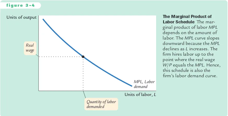
to 10 loaves per hour or less, hiring additional workers is no longer profitable. Figure 3-4 shows how the marginal product of labor depends on the amount of labor employed (holding the firm’s capital stock constant). That is, this figure graphs the MPLschedule. Because the MPL diminishes as the amount of labor
increases, this curve slopes downward. For any given real wage, the firm hires up to the point at which the MPLequals the real wage. Hence, the MPLschedule is
also the firm’s labor demand curve.
f i g u r e 3 - 4
Units of labor, L MPL, Labor demand Units of output
Quantity of labor demanded Real
wage
The Marginal Product of Labor Schedule The mar-ginal product of labor MPL
depends on the amount of labor. The MPLcurve slopes downward because the MPL
declines as Lincreases. The firm hires labor up to the point where the real wage
The Marginal Product of Capital and Capital Demand The firm decides how much capital to rent in the same way it decides how much labor to hire.The marginal product of capital (MPK)is the amount of extra output the firm gets from an extra unit of capital, holding the amount of labor constant:
MPK=F(K+1,L) −F(K,L).
Thus, the marginal product of capital is the difference between the amount of output produced with K+1 units of capital and that produced with only Kunits of capital. Like labor, capital is subject to diminishing marginal product.
The increase in profit from renting an additional machine is the extra revenue from selling the output of that machine minus the machine’s rental price:
D
Profit =D
Revenue −D
Cost=(P×MPK) −R.
To maximize profit, the firm continues to rent more capital until the MPKfalls to equal the real rental price:
MPK=R/P.
The real rental price of capitalis the rental price measured in units of goods rather than in dollars.
To sum up, the competitive, profit-maximizing firm follows a simple rule about how much labor to hire and how much capital to rent.The firm demands each factor of production until that factor’s marginal product falls to equal its real factor price.
The Division of National Income
Having analyzed how a firm decides how much of each factor to employ, we can now explain how the markets for the factors of production distribute the econ-omy’s total income. If all firms in the economy are competitive and profit maxi-mizing, then each factor of production is paid its marginal contribution to the production process.The real wage paid to each worker equals the MPL, and the real rental price paid to each owner of capital equals the MPK. The total real wages paid to labor are therefore MPL×L, and the total real return paid to cap-ital owners is MPK×K.
The income that remains after the firms have paid the factors of production is the economic profitof the owners of the firms. Real economic profit is
Economic Profit =Y−(MPL×L) −(MPK×K).
Because we want to examine the distribution of national income, we rearrange the terms as follows:
Y=(MPL×L) +(MPK×K) +Economic Profit.
How large is economic profit? The answer is surprising: if the production function has the property of constant returns to scale, as is often thought to be the case, then economic profit must be zero.That is, nothing is left after the fac-tors of production are paid.This conclusion follows from a famous mathematical result called Euler’s theorem,2which states that if the production function has con-stant returns to scale, then
F(K,L) =(MPK×K) +(MPL×L).
If each factor of production is paid its marginal product, then the sum of these factor payments equals total output. In other words, constant returns to scale, profit maximization, and competition together imply that economic profit is zero. If economic profit is zero, how can we explain the existence of “profit’’in the economy? The answer is that the term “profit’’as normally used is different from economic profit.We have been assuming that there are three types of agents: work-ers, owners of capital, and owners of firms.Total income is divided among wages, return to capital, and economic profit. In the real world, however, most firms own rather than rent the capital they use. Because firm owners and capital owners are the same people, economic profit and the return to capital are often lumped to-gether. If we call this alternative definition accounting profit, we can say that
Accounting Profit =Economic Profit +(MPK×K).
Under our assumptions—constant returns to scale, profit maximization, and competition—economic profit is zero. If these assumptions approximately de-scribe the world, then the “profit’’in the national income accounts must be mostly the return to capital.
We can now answer the question posed at the beginning of this chapter about how the income of the economy is distributed from firms to households. Each factor of production is paid its marginal product, and these factor payments ex-haust total output.Total output is divided between the payments to capital and the pay-ments to labor, depending on their marginal productivities.
2Mathematical note:To prove Euler’s theorem, begin with the definition of constant returns to scale:
zY=F(zK,zL). Now differentiate with respect to zand then evaluate at z=1.
C A S E S T U D Y
The Black Death and Factor Prices
As we have just learned, in the neoclassical theory of distribution, factor prices equal the marginal products of the factors of production. Because the marginal products depend on the quantities of the factors, a change in the quantity of any one factor alters the marginal products of all the factors. Therefore, a change in the supply of a factor alters equilibrium factor prices.
3-3
What Determines the Demand for
Goods and Services?
We have seen what determines the level of production and how the income from production is distributed to workers and owners of capital. We now con-tinue our tour of the circular flow diagram, Figure 3-1, and examine how the output from production is used.
In Chapter 2 we identified the four components of GDP:
➤ Consumption (C)
➤ Investment (I)
➤ Government purchases (G)
➤ Net exports (NX).
The circular flow diagram contains only the first three components. For now, to simplify the analysis, we assume a closed economy—a country that does not trade with other countries.Thus, net exports are always zero. (We examine the macro-economics of open economiesin Chapter 5.)
A closed economy has three uses for the goods and services it produces.These three components of GDP are expressed in the national income accounts identity:
Y=C+I+G.
Households consume some of the economy’s output;firms and households use some of the output for investment; and the government buys some of the out-put for public purposes. We want to see how GDP is allocated among these three uses.
1348 reduced the population of Europe by about one-third within a few years. Because the marginal product of labor increases as the amount of labor falls, this massive reduction in the labor force raised the marginal product of labor. (The economy moved to the left along the curves in Figures 3-3 and 3-4.) Real wages did increase substantially during the plague years—doubling, by some estimates. The peasants who were fortunate enough to survive the plague enjoyed eco-nomic prosperity.
The reduction in the labor force caused by the plague also affected the return to land, the other major factor of production in medieval Europe. With fewer workers available to farm the land, an additional unit of land produced less addi-tional output. This fall in the marginal product of land led to a decline in real rents of 50 percent or more.Thus, while the peasant classes prospered, the landed classes suffered reduced incomes.3
3
Consumption
When we eat food, wear clothing, or go to a movie, we are consuming some of the output of the economy. All forms of consumption together make up two-thirds of GDP. Because consumption is so large, macroeconomists have devoted much energy to studying how households decide how much to consume. Chap-ter 16 examines this work in detail. Here we consider the simplest story of con-sumer behavior.
Households receive income from their labor and their ownership of capital, pay taxes to the government, and then decide how much of their after-tax come to consume and how much to save. As we discussed in Section 3-2, the in-come that households receive equals the output of the economy Y. The government then taxes households an amount T. (Although the government im-poses many kinds of taxes, such as personal and corporate income taxes and sales taxes, for our purposes we can lump all these taxes together.) We define income after the payment of all taxes,Y −T, as disposable income. Households divide their disposable income between consumption and saving.
We assume that the level of consumption depends directly on the level of dis-posable income.The higher the disdis-posable income, the greater the consumption. Thus,
C=C(Y−T).
This equation states that consumption is a function of disposable income.The re-lationship between consumption and disposable income is called the consump-tion funcconsump-tion.
The marginal propensity to consume (MPC) is the amount by which
consumption changes when disposable income increases by one dollar.The MPC is between zero and one: an extra dollar of income increases consumption, but by less than one dollar. Thus, if households obtain an extra dollar of income, they save a portion of it. For example, if the MPC is 0.7, then households spend 70 cents of each additional dollar of disposable income on consumer goods and ser-vices and save 30 cents.
Figure 3-5 illustrates the consumption function. The slope of the consump-tion funcconsump-tion tells us how much consumpconsump-tion increases when disposable income increases by one dollar. That is, the slope of the consumption function is the MPC.
Investment
Both firms and households purchase investment goods. Firms buy investment goods to add to their stock of capital and to replace existing capital as it wears out. Households buy new houses, which are also part of investment.Total invest-ment in the United States averages about 15 percent of GDP.
production of goods and services) must exceed its cost (the payments for bor-rowed funds). If the interest rate rises, fewer investment projects are profitable, and the quantity of investment goods demanded falls.
For example, suppose a firm is considering whether it should build a $1 mil-lion factory that would yield a return of $100,000 per year, or 10 percent. The
firm compares this return to the cost of borrowing the $1 million. If the interest rate is below 10 percent, the firm borrows the money in financial markets and makes the investment. If the interest rate is above 10 percent, the firm forgoes the investment opportunity and does not build the factory.
The firm makes the same investment decision even if it does not have to bor-row the $1 million but rather uses its own funds.The firm can always deposit this money in a bank or a money market fund and earn interest on it. Building the factory is more profitable than the deposit if and only if the interest rate is less than the 10 percent return on the factory.
A person wanting to buy a new house faces a similar decision.The higher the interest rate, the greater the cost of carrying a mortgage. A $100,000 mortgage costs $8,000 per year if the interest rate is 8 percent and $10,000 per year if the interest rate is 10 percent. As the interest rate rises, the cost of owning a home rises, and the demand for new homes falls.
When studying the role of interest rates in the economy, economists distin-guish between the nominal interest rate and the real interest rate.This distinction is relevant when the overall level of prices is changing. The nominal interest rateis the interest rate as usually reported: it is the rate of interest that investors
pay to borrow money. The real interest rate is the nominal interest rate cor-rected for the effects of inflation. If the nominal interest rate is 8 percent and the inflation rate is 3 percent, then the real interest rate is 5 percent. In Chapter 4 we discuss the relation between nominal and real interest rates in detail. Here it is sufficient to note that the real interest rate measures the true cost of borrowing and, thus, determines the quantity of investment.
f i g u r e 3 - 5
Consumption, C
MPC
1
Consumption function
Disposable income, Y ⴚ T
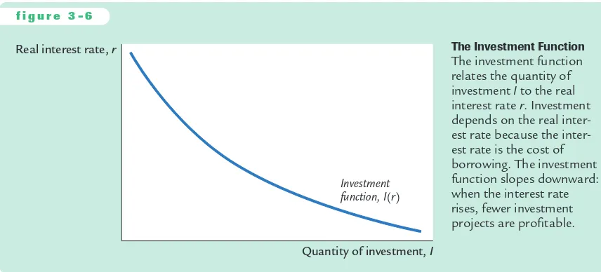
We can summarize this discussion with an equation relating investment I to the real interest rate r:
I=I(r).
Figure 3-6 shows this investment function. It slopes downward, because as the interest rate rises, the quantity of investment demanded falls.
Government Purchases
Government purchases are the third component of the demand for goods and services.The federal government buys guns, missiles, and the services of govern-ment employees. Local governgovern-ments buy library books, build schools, and hire teachers. Governments at all levels build roads and other public works. All these transactions make up government purchases of goods and services, which ac-count for about 20 percent of GDP in the United States.
These purchases are only one type of government spending.The other type is transfer payments to households, such as welfare for the poor and Social Security payments for the elderly. Unlike government purchases, transfer payments are not made in exchange for some of the economy’s output of goods and services. Therefore, they are not included in the variable G.
Transfer payments do affect the demand for goods and services indirectly. Transfer payments are the opposite of taxes: they increase households’disposable income, just as taxes reduce disposable income.Thus, an increase in transfer pay-ments financed by an increase in taxes leaves disposable income unchanged. We can now revise our definition of Tto equal taxes minus transfer payments. Dis-posable income,Y −T, includes both the negative impact of taxes and the
posi-tive impact of transfer payments.
If government purchases equal taxes minus transfers, then G=T, and the
gov-ernment has a balanced budget. If G exceeds T, the government runs a budget f i g u r e 3 - 6
Real interest rate, r
Quantity of investment, I
Investment function, I(r)
deficit, which it funds by issuing government debt—that is, by borrowing in the
financial markets. If Gis less than T, the government runs a budget surplus, which it can use to repay some of its outstanding debt.
Here we do not try to explain the political process that leads to a particular
fiscal policy—that is, to the level of government purchases and taxes. Instead, we take government purchases and taxes as exogenous variables.To denote that these variables are fixed outside of our model of national income, we write
G=G
We do, however, want to examine the impact of fiscal policy on the variables de-termined within the model, the endogenous variables.The endogenous variables here are consumption, investment, and the interest rate.
To see how the exogenous variables affect the endogenous variables, we must complete the model.This is the subject of the next section.
FYI
If you look in the business section of a newspa-per, you will find many different interest rates re-ported. By contrast, throughout this book, we will talk about “the” interest rate, as if there were only one interest rate in the economy. The only distinction we will make is between the nominal interest rate (which is not corrected for inflation) and the real interest rate (which is corrected for inflation). Almost all of the interest rates re-ported in the newspaper are nominal.
Why does the newspaper report so many in-terest rates? The various inin-terest rates differ in three ways:
➤ Term. Some loans in the economy are for short
periods of time, even as short as overnight. Other loans are for 30 years or even longer. The interest rate on a loan depends on its term. Long-term interest rates are usually, but not always, higher than short-term interest rates.
➤ Credit risk. In deciding whether to make a loan,
a lender must take into account the probabil-ity that the borrower will repay. The law allows borrowers to default on their loans by declar-ing bankruptcy. The higher the perceived
prob-The Many Different Interest Rates
ability of default, the higher the interest rate. The safest credit risk is the government, and so government bonds tend to pay a low interest rate. At the other extreme, financially shaky corporations can raise funds only by issuing
junk bonds, which pay a high interest rate to compensate for the high risk of default.
➤ Tax treatment. The interest on different types of
bonds is taxed differently. Most important, when state and local governments issue bonds, called municipal bonds, the holders of the bonds do not pay federal income tax on the interest income. Because of this tax advan-tage, municipal bonds pay a lower interest rate.
When you see two different interest rates in the newspaper, you can almost always explain the difference by considering the term, the credit risk, and the tax treatment of the loan.
3-4
What Brings the Supply and Demand for
Goods and Services Into Equilibrium?
We have now come full circle in the circular flow diagram, Figure 3-1. We began by examining the supply of goods and services, and we have just dis-cussed the demand for them. How can we be certain that all these flows bal-ance? In other words, what ensures that the sum of consumption, investment, and government purchases equals the amount of output produced? We will see that in this classical model, the interest rate has the crucial role of equilibrating supply and demand.
There are two ways to think about the role of the interest rate in the econ-omy. We can consider how the interest rate affects the supply and demand for goods or services. Or we can consider how the interest rate affects the supply and demand for loanable funds. As we will see, these two approaches are two sides of the same coin.
Equilibrium in the Market for Goods and Services:
The Supply and Demand for the Economy
’
s Output
The following equations summarize the discussion of the demand for goods and services in Section 3-3:
Y=C+I+G.
C=C(Y−T).
I=I(r).
G=G
_
.
T=T
_
.
The demand for the economy’s output comes from consumption, investment, and government purchases. Consumption depends on disposable income; invest-ment depends on the real interest rate; and governinvest-ment purchases and taxes are the exogenous variables set by fiscal policymakers.
To this analysis, let’s add what we learned about the supply of goods and ser-vices in Section 3-1.There we saw that the factors of production and the pro-duction function determine the quantity of output supplied to the economy:
Y=F(K–,L–) =Y–.
Now let’s combine these equations describing the supply and demand for output. If we substitute the consumption function and the investment function into the national income accounts identity, we obtain
Because the variables G and Tare fixed by policy, and the level of output Y is
fixed by the factors of production and the production function, we can write
Y–=C(Y–−T–) +I(r) +G–.
This equation states that the supply of output equals its demand, which is the sum of consumption, investment, and government purchases.
Notice that the interest rate ris the only variable not already determined in the last equation. This is because the interest rate still has a key role to play: it must adjust to ensure that the demand for goods equals the supply.The greater the interest rate, the lower the level of investment, and thus the lower the de-mand for goods and services,C+I +G. If the interest rate is too high, invest-ment is too low, and the demand for output falls short of the supply. If the interest rate is too low, investment is too high, and the demand exceeds the supply.At the equilibrium interest rate, the demand for goods and services equals the supply.
This conclusion may seem somewhat mysterious. One might wonder how the interest rate gets to the level that balances the supply and demand for goods and services.The best way to answer this question is to consider how financial mar-kets fit into the story.
Equilibrium in the Financial Markets:
The Supply and Demand for Loanable Funds
Because the interest rate is the cost of borrowing and the return to lending in fi -nancial markets, we can better understand the role of the interest rate in the economy by thinking about the financial markets.To do this, rewrite the national income accounts identity as
Y−C−G=I.
The term Y−C−Gis the output that remains after the demands of consumers and the government have been satisfied; it is called national savingor simply
saving(S). In this form, the national income accounts identity shows that saving equals investment.
To understand this identity more fully, we can split national saving into two parts—one part representing the saving of the private sector and the other repre-senting the saving of the government:
(Y−T−C) +(T−G) =I.
diagram in Figure 3-1 reveals an interpretation of this equation: this equation states that the flows into the financial markets (private and public saving) must balance the flows out of the financial markets (investment).
To see how the interest rate brings financial markets into equilibrium, substi-tute the consumption function and the investment function into the national in-come accounts identity:
Y−C(Y−T) −G=I(r).
Next, note that Gand Tare fixed by policy and Yis fixed by the factors of pro-duction and the propro-duction function:
Y–−C(Y–−T–) −G–=I(r) S–=I(r).
The left-hand side of this equation shows that national saving depends on in-come Yand the fiscal-policy variables Gand T. For fixed values of Y,G, and T, national saving Sis also fixed.The right-hand side of the equation shows that in-vestment depends on the interest rate.
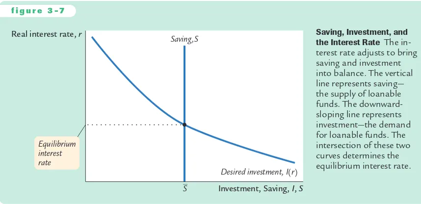
Figure 3-7 graphs saving and investment as a function of the interest rate.The saving function is a vertical line because in this model saving does not depend on the interest rate (although we relax this assumption later).The investment func-tion slopes downward: the higher the interest rate, the fewer profitable invest-ment projects.
From a quick glance at Figure 3-7, one might think it was a supply-and-demand diagram for a particular good. In fact, saving and investment can be in-terpreted in terms of supply and demand. In this case, the “good’’is loanable funds, and its “price’’is the interest rate. Saving is the supply of loanable funds—
f i g u r e 3 - 7
Real interest rate, r
S Saving ,S
Investment, Saving, I, S Desired investment, I(r) Equilibrium
interest rate
Saving, Investment, and the Interest Rate The in-terest rate adjusts to bring saving and investment into balance. The vertical line represents saving—
households lend their saving to investors or deposit their saving in a bank that then loans the funds out. Investment is the demand for loanable funds—investors borrow from the public directly by selling bonds or indirectly by borrowing from banks. Because investment depends on the interest rate, the quantity of loanable funds demanded also depends on the interest rate.
The interest rate adjusts until the amount that firms want to invest equals the amount that households want to save. If the interest rate is too low, in-vestors want more of the economy’s output than households want to save. Equivalently, the quantity of loanable funds demanded exceeds the quantity supplied. When this happens, the interest rate rises. Conversely, if the interest rate is too high, households want to save more than firms want to invest; be-cause the quantity of loanable funds supplied is greater than the quantity de-manded, the interest rate falls. The equilibrium interest rate is found where the two curves cross.At the equilibrium interest rate, households’desire to save bal-ances firms’desire to invest, and the quantity of loanable funds supplied equals the quantity demanded.
Changes in Saving: The Effects of Fiscal Policy
We can use our model to show how fiscal policy affects the economy.When the government changes its spending or the level of taxes, it affects the demand for the economy’s output of goods and services and alters national saving, invest-ment, and the equilibrium interest rate.
An Increase in Government Purchases Consider first the effects of an in-crease in government purchases of an amount
D
G. The immediate impact is to increase the demand for goods and services byD
G. But since total output isfixed by the factors of production, the increase in government purchases must be met by a decrease in some other category of demand. Because disposable income
Y −Tis unchanged, consumption Cis unchanged.The increase in government purchases must be met by an equal decrease in investment.
To induce investment to fall, the interest rate must rise. Hence, the increase in government purchases causes the interest rate to increase and investment to de-crease. Government purchases are said to crowd outinvestment.
f i g u r e 3 - 8
Real interest rate, r
I(r)
Investment, Saving, I, S
r2
r1
S2 S1
1. A fall in saving . . . 2. . . . raises
the interest rate . . .
A Reduction in Saving A reduction in saving, possi-bly the result of a change in fiscal policy, shifts the saving schedule to the left. The new equilibrium is the point at which the new saving schedule crosses the investment schedule. A re-duction in saving lowers the amount of investment and raises the interest rate. Fiscal-policy actions that reduce saving are said to crowd out investment.
C A S E S T U D Y
Wars and Interest Rates in the United Kingdom, 1730–1920 Wars are traumatic—both for those who fight them and for a nation’s economy. Because the economic changes accompanying them are often large, wars provide a natural experiment with which economists can test their theories.We can learn about the economy by seeing how in wartime the endogenous variables respond to the major changes in the exogenous variables.
One exogenous variable that changes substantially in wartime is the level of government purchases. Figure 3-9 shows military spending as a percentage of GDP for the United Kingdom from 1730 to 1919. This graph shows, as one would expect, that government purchases rose suddenly and dramatically during the eight wars of this period.
Our model predicts that this wartime increase in government purchases—and the increase in government borrowing to finance the wars—should have raised the demand for goods and services, reduced the supply of loanable funds, and raised the interest rate.To test this prediction, Figure 3-9 also shows the interest rate on long-term government bonds, called consols in the United Kingdom. A positive association between military purchases and interest rates is apparent in this figure. These data support the model’s prediction: interest rates do tend to rise when government purchases increase.4
A Decrease in Taxes Now consider a reduction in taxes of
D
T. The immediate impact of the tax cut is to raise disposable income and thus to raise consumption. Disposable income rises byD
T, and consumption rises by an amount equal to One problem with using wars to test theories is that many economic changes may be occurring at the same time. For example, in World War II, while government purchases increased dramatically, rationing also restricted consumption of many goods. In addition, the risk of defeat in the war and default by the government on its debt presumably increases the interest rate the government must pay. Economic models predict what happens when one exogenous variable changes and all the other exogenous variables remain constant. In the real world, however, many exoge-nous variables may change at once. Unlike controlled laboratory experiments, the natural experiments on which economists must rely are not always easy to interpret.f i g u r e 3 - 9
Seven Years War Boer War
World
1730 1750 1770 1790 1810 1830
Year
Military Spending and the Interest Rate in the United Kingdom This figure shows
military spending as a percentage of GDP in the United Kingdom from 1730 to 1919. Not surprisingly, military spending rose substantially during each of the eight wars of this period. This figure also shows that the interest rate tended to rise when military spending rose.
D
Ttimes the marginal propensity to consume MPC. The higher the MPC, the greater the impact of the tax cut on consumption.Because the economy’s output is fixed by the factors of production and the level of government purchases is fixed by the government, the increase in con-sumption must be met by a decrease in investment. For investment to fall, the in-terest rate must rise. Hence, a reduction in taxes, like an increase in government purchases, crowds out investment and raises the interest rate.
We can also analyze the effect of a tax cut by looking at saving and invest-ment. Because the tax cut raises disposable income by
D
T, consumption goes upby MPC ×
D
T. National saving S, which equals Y − C − G, falls by the same amount as consumption rises. As in Figure 3-8, the reduction in saving shifts the supply of loanable funds to the left, which increases the equilibrium interest rate and crowds out investment.Changes in Investment Demand
So far, we have discussed how fiscal policy can change national saving. We can also use our model to examine the other side of the market—the demand for in-vestment. In this section we look at the causes and effects of changes in invest-ment demand.
One reason investment demand might increase is technological innovation. Suppose, for example, that someone invents a new technology, such as the rail-road or the computer. Before a firm or household can take advantage of the in-novation, it must buy investment goods. The invention of the railroad had no value until railroad cars were produced and tracks were laid. The idea of the computer was not productive until computers were manufactured.Thus, techno-logical innovation leads to an increase in investment demand.
Investment demand may also change because the government encourages or discourages investment through the tax laws. For example, suppose that the gov-ernment increases personal income taxes and uses the extra revenue to provide tax cuts for those who invest in new capital. Such a change in the tax laws makes more investment projects profitable and, like a technological innovation, in-creases the demand for investment goods.
Figure 3-10 shows the effects of an increase in investment demand. At any given interest rate, the demand for investment goods (and also for loanable funds) is higher. This increase in demand is represented by a shift in the investment schedule to the right.The economy moves from the old equilibrium, point A, to the new equilibrium, point B.
The surprising implication of Figure 3-10 is that the equilibrium amount of investment is unchanged. Under our assumptions, the fixed level of saving deter-mines the amount of investment; in other words, there is a fixed supply of loan-able funds. An increase in investment demand merely raises the equilibrium interest rate.
depend on the interest rate. Because the interest rate is the return to saving (as well as the cost of borrowing), a higher interest rate might reduce consumption and increase saving. If so, the saving schedule would be upward sloping, rather than vertical.
With an upward-sloping saving schedule, an increase in investment demand would raise both the equilibrium interest rate and the equilibrium quantity of investment. Figure 3-11 shows such a change. The increase in the interest rate causes households to consume less and save more.The decrease in consumption frees resources for investment.
f i g u r e 3 - 1 0
Real interest rate, r
Investment, Saving, I, S An increase in the demand for investment goods shifts the investment schedule to the right. At any given interest rate, the amount of investment is greater. The equilibrium moves from point A to point B. Because the amount of saving is fixed, the increase in investment demand
Real interest rate, r
2. . . . raises
Rate When saving is
3-5
Conclusion
In this chapter we have developed a model that explains the production, dis-tribution, and allocation of the economy’s output of goods and services. Be-cause the model incorporates all the interactions illustrated in the circular flow diagram in Figure 3-1, it is sometimes called a general equilibrium model. The model emphasizes how prices adjust to equilibrate supply and demand. Factor prices equilibrate factor markets.The interest rate equilibrates the sup-ply and demand for goods and services (or, equivalently, the supsup-ply and de-mand for loanable funds).
FYI
In our model, investment depends on the interest rate. The higher the interest rate, the fewer in-vestment projects there are that are profitable. The investment schedule therefore slopes down-ward.
Economists who look at macroeconomic data, however, usually fail to find an obvious as-sociation between investment and interest rates. In years when interest rates are high, investment is not always low. In years when interest rates are low, investment is not always high.
How do we interpret this finding? Does it mean that investment does not depend on the in-terest rate? Does it suggest that our model of saving, investment, and the interest rate is incon-sistent with how the economy actually functions? Luckily, we do not have to discard our model. The inability to find an empirical relationship be-tween investment and interest rates is an example
of the identification problem. The identification
problem arises when variables are related in more than one way. When we look at data, we are observing a combination of these different relationships, and it is difficult to “identify’’ any one of them.
To understand this problem more concretely, consider the relationships among saving, invest-ment, and the interest rate. Suppose, on the one hand, that all changes in the interest rate re-sulted from changes in saving—that is, from
The Identification Problem
shifts in the saving schedule. Then, as shown in the left-hand side of panel (a) in Figure 3-12, all changes would represent movement along a fixed investment schedule. As the right-hand side of panel (a) shows, the data would trace out this in-vestment schedule. Thus, we would observe a negative relationship between investment and in-terest rates.
Suppose, on the other hand, that all changes in the interest rate resulted from technological innovations—that is, from shifts in the invest-ment schedule. Then, as shown in panel (b), all changes would represent movements in the in-vestment schedule along a fixed saving schedule. As the right-hand side of panel (b) shows, the data would reflect this saving schedule. Thus, we would observe a positive relationship between in-vestment and interest rates.
Throughout the chapter, we have discussed various applications of the model. The model can explain how income is divided among the factors of production and how factor prices depend on factor supplies.We have also used the model to
discuss how fiscal policy alters the allocation of output among its alternative
uses—consumption, investment, and government purchases—and how it affects
the equilibrium interest rate.
What,s Happening What We Observe
(b) Shifting Investment Schedules
r
I, S r
I, S
What,s Happening What We Observe
(c) Shifting Saving Schedules and Investment Schedules
r
I, S r
I, S
What,s Happening What We Observe
Identifying the Investment Function
At this point it is useful to review some of the simplifying assumptions we have made in this chapter. In the following chapters we relax some of these as-sumptions in order to address a greater range of questions.
➤ We have ignored the role of money, the asset with which goods and
ser-vices are bought and sold. In Chapter 4 we discuss how money affects the economy and the influence of monetary policy.
➤ We have assumed that there is no trade with other countries. In Chapter 5
we consider how international interactions affect our conclusions.
➤ We have assumed that the labor force is fully employed. In Chapter 6 we
examine the reasons for unemployment and see how public policy infl u-ences the level of unemployment.
➤ We have assumed that the capital stock, the labor force, and the production
technology are fixed. In Chapters 7 and 8 we see how changes over time in each of these lead to growth in the economy’s output of goods and ser-vices.
➤ We have ignored the role of short-run sticky prices. In Chapters 9 through
13, we develop a model of short-run fluctuations that includes sticky prices.We then discuss how the model of short-run fluctuations relates to the model of national income developed in this chapter.
Before going on to these chapters, go back to the beginning of this one and make sure you can answer the four groups of questions about national income that begin the chapter.
Summary
1.The factors of production and the production technology determine the
economy’s output of goods and services. An increase in one of the factors of production or a technological advance raises output.
2.Competitive, profit-maximizing firms hire labor until the marginal product
of labor equals the real wage. Similarly, these firms rent capital until the mar-ginal product of capital equals the real rental price. Therefore, each factor of production is paid its marginal product. If the production function has con-stant returns to scale, all output is used to compensate the inputs.
3.The economy’s output is used for consumption, investment, and government
purchases. Consumption depends positively on disposable income. Invest-ment depends negatively on the real interest rate. GovernInvest-ment purchases and taxes are the exogenous variables of fiscal policy.
4.The real interest rate adjusts to equilibrate the supply and demand for the